02050534 - Cafet Innova

www.cafetinnova.orgIndexed inScopus Compendex and Geobase Elsevier, ChemicalAbstract Services-USA, Geo-Ref Information Services-USAISSN 0974-5904, Volume 05, No. 05 (01)October 2012, P.P. 1358-1370Road Traffic Noise Assessment and Modeling in Bhubaneswar,India: A Comparative and Comprehensive Monitoring StudyBIJAY KUMAR SWAIN 1 , SHREERUP GOSWAMI 2 and SANTOSH KUMAR PANDA 31 Department of Environmental Science, Utkal University, Bhubaneswar-751004, Odisha, India2 Department of Geology, Ravenshaw University, Cuttack-753003, Odisha, India3 Department of Physics, Dr. J.N.College, Rasalpur, Balasore-756021, Odisha, IndiaEmail: swainbijay0@gmail.com, goswamishreerup@gmail.com, skpanda_physics@yahoo.comAbstract: The road traffic noise environment in Bhubaneswar, one of the important cities of eastern India, capital ofthe Odisha State, in terms of standard noise indices were worked out in the present study. Noise pollution wasanalysed in 16 different squares (road sections) during six different specified times (7-10 a.m., 11a.m.-2 p.m., 3-6p.m., 7-10 p.m., 10 p.m.-1 a.m., 3a.m.-6 a.m.) to assess the level of noise pollution of the city. The sources of noiseat the studied sites were predominantly attributable to motor vehicular traffic. Noise descriptors such as L 10 , L 50 , L 90 ,Leq, TNI (Traffic Noise Index), NPL (Noise Pollution Level) and NC (Noise climate) were assessed to reveal theextent of noise pollution due to crowded and busy traffic in this capital city. L 10 , L 50, L 90, L eq , NPL, TNI and NCvalues of all 16 monitored sites ranged from 75.6 to 82.7 dB, from 67.2 to 74.2 dB, from 61.1 to 67.7 dB, from 70.4to 80.6 dB; from 83 to 101.1 dB, from 80.7 to 113.1 dB, and from 12 to 20.5 dB during day time, while L 10 , L 50 , L 90 ,Leq, NPL, TNI, NC values ranged from 74.2 to 79.3 dB; 61.2 to 64.1 dB; 55.7 to 60.3 dB; 66.9 to 71.7 dB; 82.7 to94.5 dB; 91 to 116.9 dB and 15.8 to 22.8 dB, respectively during night time. The present noise assessment depictedthat even the minimum values of Leq (70.4 dB), NPL (83 dB), TNI (80.7 dB) during day time were more than thepermissible limit (70 dB). Lden varied from 70.2 to 73.6 dB. Chi-square (χ 2 ) test was also computed for investigatedsquares at the peak hour i.e. 7-10 p.m. to infer the level of significance. The numbers of vehicles passing through afixed point on the studied road are counted to assess the traffic volume (Q) and the percentage of heavy trucks andbuses to total traffic was also calculated to work out truck traffic mix ratio (P). Comparison of predicted/simulatednoise level with that of the actual measured data demonstrated that the model used for the prediction has the abilityto calibrate the multi-component traffic noise and yield reliable results close to that by direct measurement.Moreover, individual contribution to environmental noise by the air horn of different motor vehicles has beenassessed in and around this city during day time. The episodic and impulsive noise levels of different types ofvehicles were more than the traffic noise-limit i.e. 70 dB (A). An extensive survey adopting questionnaire methodamongst 539 local inhabitants had also been carried out to gather information about the suffering of people.Keywords: Bhubaneswar, Community Response, Modeling, Noise Descriptors, Road Traffic Noise.Introduction:Various noise surveys conclusively reveal that the busyroad traffic is the predominant source of annoyance; noother single noise has been of comparable importance(Goswami, 2009; 2011; Goswami et al., 2011; Banerjeeand Chakraborty, 2006; Chakraborty et al., 2002). InIndia, some studies on the traffic noise monitoring havebeen carried out at different cities like Delhi (Kumarand Jain, 1994; Singh and Jain, 1995; Nirjar et al., 2003,Kumar et al., 2004; Prakash et al., 2006), Mumbai(Dixit et al., 1982; Naik, 1998), Aurangabad (Bhosale etal., 2010), Amravati (Patil et al., 2011), Dehradun(Ziaudin et al., 2007), Lucknow (Kisku et al., 2006),Varanasi (Pathak et al., 2008; Tripathi et al., 2006),Jaipur (Agarwal and Swami, 2009a; 2009b; Agarwal etal., 2009; Choudhary et al., 2003), Guwahati (Deka,2000); Kolkata (Roy et al., 1984; Chakraborty et al.,2002), Asansol (Banerjee and Chakraborty, 2006;Banerjee et al., 2008; 2009), Bolpur (Padhy and Padhi,2008), Burdwan (Datta et al., 2006), Visakhapatnam(Rao et al., 1987; Rao and Rao, 1992), Anantpur(Ravindranath et al., 1989), Chennai (Kalai Selvi andRamachandraiah, 2009), Thiruvanatapuram, Kochi,Kozhikode (Sampath et al., 2004), Jharsuguda (Patel etal., 2006); Bhadrak (Goswami, 2011; Swain et al.,2012) and Balasore (Goswami, 2009; Goswami et. al.,2011; Goswami and Swain, 2011) etc. and the averagenoise levels in these cities have been found to be morethan the recommended value. Particularly in Odisha,due to rapid industrial and economic growth, thetransportation sector is growing rapidly and the numberof vehicles on roads is increasing at a faster rate. Thishas led to overcrowded roads and pollution. Heavy#02050534 Copyright ©2012 CAFET-INNOVA TECHNICAL SOCIETY. All rights reserved.

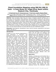
1359Road Traffic Noise Assessment and Modeling in Bhubaneswar,India: A Comparative and Comprehensive Monitoring Studytraffic volumes, higher speeds, and greater number oftrucks and buses in general and motor bikes in particularcreate enormous noise. Improper stoppage of buses atlocations rather than desired bus stoppage, improperparking of four wheelers along the road also causetraffic jams (Agarwal and Swami, 2011). Thepopulation of studied Bhubaneswar city, capital ofOdisha was only 8170 in 1921, which reached 9,04,721in 2011 census. The demographic characteristics ofBhubaneswar are presented in Table 1. It clearlydepicted that the increase in population of Bhubaneswarwas faster especially after 1991. An emerging IT(Information Technology) hub, the boom in the metalsand metal processing industries, an educational hubcomprising nine universities, few hundreds ofengineering, medical, management, general collegeshave made Bhubaneswar as one of the fastestdeveloping cities of India in recent years. Thus, thevehicular density has been also increasing in last fewyears. Thus, an attempt has been made in this study torecord the road traffic noise levels at 16 differentsquares (major intersection points) to assess the extentof vehicular noise pollution around Bhubaneswar, thecapital city of the state of Odisha. For the first time,collectively, all aspects of noise monitoring survey weredealt in the present study. Most of the noise descriptors(Lmax, Lmin, Lmean, L 10 , L 50 , L 90 , Leq, NPL, TNI, NC,traffic volume-Q, truck traffic mix ratio-P) and episodicand impulsive noise levels produced by the air horn ofdifferent motor vehicles were assessed. Noise predictionmodel was applied, and measured and simulated valueswere compared. So this was one of the mostcomprehensive studies on road traffic noise ever workedout in India.Materials and Method:Acoustic Study:The studied Bhubaneswar city is located at 20° 15' NLatitude and 85° 52' E Longitude (Fig. 1). Thegeographical area of this city is around 135 sq. km.Noise levels were measured following standardprocedure using calibrated sound level (dB) meter(Model LUTREN, SL-4010) in between the months ofApril and June, 2011 at sixteen important and crowdedsquares (road sections) of Bhubaneswar (Ram mandirsquare, Gopabandhu square, Rupali square, Khandagirisquare, Rasulgarh square, Barmunda square, CRPsquare, Vani Vihar square, AG square, Master Canteensquare, Rajmahal square, Jaydev Vihar square, Kalpanasquare, Forest park square, State Museum square andRabitalkies square) (Pamanikabud and Chairasi, 1999;Ouis 2001; Kudesia and Tiwari, 2007; Ghatass, 2009;Swain et al., 2011; Goswami and Swain, 2012;Mohapatra and Goswami, 2012 a, b). Sixtymeasurements were made within one hour duration (i.e.at one minute interval) during six specified times i.e.from 7 a.m.-10 a.m., 11 a.m.-2 p.m., 3 p.m.-6 p.m., 7p.m.-10 p.m., 10 p.m.-1 a.m., 3 a.m.-6.a.m.. The noisemonitoring was done in a good climatic condition,(where there was no sign for cloud) in all working daysexcluding Sunday and local holidays in order to getbetter result.Equivalent Noise Level (Leq):Leq represents the equivalent energy sound level of asteady state and invariable sound. It includes bothintensity and length of all sounds occurring during agiven period. The noise levels of different squares indifferent time intervals were predicted along with theirequivalent noise levels (L eq ). The value of L eq in dB (A)unit is calculated by using the formula of Robinson,1971, i.e.,L eq = L 50 + (L 10 -L 90 ) 2 / 56For the present study the different percentile noiselevels used are:L 10 : The level that were exceeded during 10% of themeasuring time in dB(A).L 50 : The level that were exceeded during 50% of themeasuring time in dB(A).L 90 : The level that were exceeded during 90% of themeasuring time in dB(A).Noise Pollution Level (NPL):As L eq is an insufficient descriptor of the annoyancecaused by fluctuating noise (Robinson, 1971), NoisePollution Level (NPL) expressed in dB is calculated byusing the following formula:NPL = L eq + a (L 10 -L 90 )Where a = 1.0 (constant in the equation).NPL takes into account the variations in the soundsignal and hence serves as better indicator of thepollution in the environment for physiological andpsychological disturbance of the human system.Traffic Noise Index (TNI):Traffic Noise Index (TNI) is another parameter, whichindicates the degree of variation in a traffic flow. This isalso expressed in dB (A) and can be computed using thefollowing relation:TNI = 4 (L 10 -L 90 ) + L 90 – 30 dB (A)Noise Climate (NC):Noise Climate (NC) is the range over which the soundlevels are fluctuating in an interval of time and isassessed using the following formula:NC = (L 10 -L 90 )Where L 90 , the level exceeded for 90 % of the time ofrecord, is very near to the background noise level in theabsence of any motor vehicle trafficInternational Journal of Earth Sciences and EngineeringISSN 0974-5904, Vol. 05, No. 05 (01), October 2012, pp. 1358-1370

1361Road Traffic Noise Assessment and Modeling in Bhubaneswar,India: A Comparative and Comprehensive Monitoring Studytime (Table 2a) and from 52.1 to 101.3 dB; 52.6 to100.1 dB; 52.1 to 98.6 dB; 51.6 to 99.4 dB; 51.4 to 99.1dB; 50.6 to 98.7 dB; 51.8 to 99.5 dB; 52.5 to 96.3 dB;52.2 to 100.7 dB; 51.8 to 100.7 dB; 50.9 to 100.8 dB;55.4 to 99.2 dB; 54.3 to 98.9 dB; 52.6 to 96.3 dB; 51.3to 96.4 dB; 51.8 to 100.3 dB respectively, during nighttime (Table 2b).L 10 values of all 16 monitored sites ranged from 75.6 to81.5 dB; 75.6 to 82.5 dB; 75.6 to 82.5 dB; 75.8 to 82.7dB; 76.8 to 79.3 dB; 74.2 to 79.2 dB during 7 a.m.-10a.m., 11 a.m.-2 p.m., 3 p.m.-6 p.m., 7 p.m.-10 p.m., 10p.m.-1 a.m., 3 a.m.-6 a.m., respectively (Tables 2a, 2b).Similarly, L 50 and L 90 values of all 16 monitored sitesvaried from 67.6 to 73.1 dB and 61.3 to 67.7 dB; 67.3 to73.6 dB and 61.5 to 65.8 dB; 67.6 to 74.2 dB and 61.1to 64.6 dB; 67.2 to 74.2 dB and 61.5 to 65.2 dB; 61.3 to64.1 dB and 55.7 to 60.3 dB; 61.2 to 63.6 dB and 56.6to 59.6 dB during 7 a.m.-10 a.m., 11 a.m.-2 p.m., 3p.m.-6 p.m., 7 p.m.-10 p.m., 10 p.m.-1 a.m., 3 a.m.-6a.m., respectively (Tables 2a, 2b). Accordingly, thecalculated Leq (equivalent noise levels) values rangedfrom 70.6 to 77.7 dB; 70.4 to 78.5 dB; 71.2 to 80.6 dB;70.9 to 79.6 dB; 66.9 to 71.7 dB and 67.1 to 70.6 dBduring 7 a.m.-10 a.m., 11 a.m.-2 p.m., 3 p.m.-6 p.m., 7p.m.-10 p.m., 10 p.m.-1 a.m., 3 a.m.-6 a.m., respectively(Table 4; Table 2b). NPL values of all 16 monitoredsites ranged from 83.7 to 94.1 dB; 83 to 96.2 dB; 85.5 to101.1 dB; 85.4 to 98.5 dB; 82.7 to 94.5 dB and 83.1 to91.8 dB during 7 a.m.-10 a.m., 11 a.m.-2 p.m., 3 p.m.-6p.m., 7 p.m.-10 p.m., 10 p.m.-1 a.m., 3 a.m.-6 a.m.,respectively (Table 3). TNI values ranged from 80.7 to101.7 dB; 81.9 to 106 dB; 86.9 to 113.1 dB; 88.1 to108.7 dB; 91 to 116.9 dB and 92.2 to 114.2 dB during 7a.m.-10 a.m., 11 a.m.-2 p.m., 3 p.m.-6 p.m., 7 p.m.-10p.m., 10 p.m.-1 a.m., 3 a.m.-6 a.m., respectively, whileNC values ranged from 12 to 16.8 dB; 12.1 to 17.9 dB;13.7 to 20.5 dB; 13.8 to 19.1 dB; 15.8 to 22.8 dB and 16to 21.9 dB during 7 a.m.-10 a.m., 11 a.m.-2 p.m., 3p.m.-6 p.m., 7 p.m.-10 p.m., 10 p.m.-1 a.m., 3 a.m.-6a.m., respectively (Table 3). All these values clearlyshow high noise levels in Bhubaneswar city mostlythroughout the evening time starting from 7 p.m. to 10p.m..The present noise assessment depicted that even theminimum values of Leq (70.4 dB), NPL (83 dB), TNI(80.7 dB) during day time were more than thepermissible limit (70 dB). It was also observed that atsome locations the characteristics of noise caused byfast moving traffic, different from those caused bycongested or slow moving traffic. Noise from congestedtraffic was found to contain occasional peaks and varymore in levels. A systematic comparison between TNIand Leq noise levels for all selected locations revealedthat the TNI values were much more than respectiveLeq levels. This simply demonstrated that although thenoise levels during any period of the day were generallyconstant but the presence of single – event noise wassufficient to affect the values of different noisepercentile levels and consequently the TNI. This is dueto overpopulated road ways with bad conditions, brokenroads, minimal traffic management and hootingbehavior of drivers (Agarwal and Swami, 2009).The calculated χ 2 values are 0.789; 1.286; 2.575 and2.354 for different time intervals such as 7 a.m.-10 a.m.,11 a.m.-2 p.m., 3 p.m.-6 p.m. and 7 p.m.-10 p.m.But χ 2 tabulated at 99% level of significance at 15 degreesof freedom = 5.229χ 2 tabulated at 97% level of significance at 15 degrees offreedom = 6.262χ 2 tabulated at 95% level of significance at 15 degrees offreedom = 7.261χ 2 tabulated at 5% level of significance at 15 degrees offreedom = 24.996Since our χ 2 values are very less in comparison totabulated values of χ 2 , therefore, χ 2 calculated and χ 2 observedvalues are in good agreement at 15 degrees of freedomand at 99, 97, 95 and 5 % levels of significance.For validation of the road traffic noise prediction modelgiven by Griffith and Langdon (1968), calculated Leq iscompared with the observed Leq values. Table 4compares the measured noise levels against thosecalculated using the aforesaid model. The Co-relation(R 2 ) value for observed Leq versus calculated Leq forthe present model is 0.94, 0.812, 0.823 and 0.96 fordifferent time intervals (7 a.m.-10 a.m., 11 a.m.-2 p.m.,3 p.m.-6 p.m., 7 p.m.-10 p.m.) of the aforesaid squares.Using the given data, this model has been checked forvalidation by R 2 value and χ 2 test, which have givengood results. It demonstrates that the monitored valuesare more or less same with predicted values. Hence thismodel can be used for noise prediction for Indianconditions.Every day, thousands of auto-rickshaws, two wheelersand cars, hundreds of buses, cargo carrying trucks anddumpers run along these roads. A comparative data onthe number of different types of vehicles passes throughthe studied traffic squares in a day is presented in theTable 5. Maximum number of total vehicles passing inunit time was observed at Baramunda square (14605)followed by Rasulgarh square (14521), Jayadev Viharsquare (14187) and Rabi Talkies square (14140),whereas minimum number of total vehicles passing inunit time was observed at State Museum square(10653), Forest park square (10847), Rupali square(11150), Gopabandhu square (11297) and AG square(11342) (Table 5). The number of vehicles passingthrough a fixed point on the studied road is counted toassess the traffic volume (Q) (Table 6). The trafficvolume is maximum (1326) at Rasulgarh square duringInternational Journal of Earth Sciences and EngineeringISSN 0974-5904, Vol. 05, No. 05 (01), October 2012, pp. 1358-1370

BIJAY KUMAR SWAIN, SHREERUP GOSWAMI and SANTOSH KUMAR PANDA13627-10 p.m., followed by 1308 at Barmunda square during7-10 p.m. and 1290 at Khandagiri square during 7-10p.m.. It was observed that noise levels were increasingwith increased traffic volume. The percentage of heavytrucks and buses to total traffic is calculated to work outtruck traffic mix ratio (P) (Table 6). Similarly, trucktraffic mix ratio (P) was maximum (14.97) atRabitalkies square during 7-10 p.m., followed by 14.95at Rabitalkies square during 11 a.m.-2 p.m. and 14.37during 7-10 p.m. at Barmunda square. These data revealthat an increase in this ratio increases the noise level.Lden values of the above said sixteen road sections ofthe capital city, Bhubaneswar ranged from 70.2 to 73.6dB (Table 7). Even Lden is also more than day timepermissible limit of road traffic noise. Thus, it is evidentthat the noise pollution in and around aforesaid sixteensquares of Bhubaneswar city throughout the day andevening is upsetting.The exercise to point out the type of vehicles and itscontribution to environmental noise brought outinteresting findings. The objectives of measuring thenoise levels firstly was to have an estimate of itsindividual contribution to the environmental noise andsecondly to reflect the maintenance levels of thevehicles prevalent in the area. The vehicular noise levelsof Bhubaneswar were depicted in the Table 8. It isobserved that the trucks (129 dB) are producing morenoise followed by college bus (128.8 dB). Noiseproduced from motor cycles, town buses, mini trucks,cars and tempos ranged between 97.8 and 116.1 dB;111.7 and 127.7 dB; 105.6 and 118.4 dB; 105.9 and117.4 dB; 105.6 and 119.4 dB, respectively and thenoise levels for other vehicles were also given (Table 8).However, the peak traffic was observed during 7-10p.m. at all the monitoring squares of the city. Maximumnumbers of peoples are traveling during the morningand evening time for office work and schools havingsimilar working hours. High frequency sound emittedfromelectric horn and air horn of buses, trucks, cars,motorcycles, auto-rickshaws, engine of vehicles,crowding of general public create tremendous noise.The present study explicitly demonstrated that in mostof the cases, the average assessed sound pressure levelswere more than the permissible limit (70 dB for roadtraffic noise) (WHO, 1999; Krishna Murthy et al.,2007). The whole population of Bhubaneswar includingthousands of floating population coming to this capitalcity for different purposes from nearby hundreds ofsmall towns and villages are exposed to this urban noiselevels of more than 70.0 dB (A). This is a very highlevel, corresponding to the day time limit recommendedby the WHO for urban centers (55 dB).Community Response:The noise perception survey was carried out by aquestionnaire, which was administered to 539individuals in Bhubaneswar during May, 2011. Thissurvey clearly demonstrates that most of the peoplewere aware of noise pollution but its adverse healtheffect was not fully realized. 67 % respondents were notsatisfied about the noise level at Bhubaneswar. Themost imperative finding was that traffic noise wasranked in first place among the most frequentlyidentified types of sound and was considered unpleasantby the majority (79%). The reasons for noise pollutionwere evaluated as Horn (56%) followed by traffic jam(20%), silencer (13%) and engine (11%). Majority ofthe respondents (56%) were irritated with the air-hornnoise from motor cycle and auto-rickshaw. 39 %respondents identified headache as the main healtheffect of noise pollution. 23% interviewees were feelingmental stress, 11% were suffering from insomnia and0.1% respondents were suffering from hearing loss. Theperiods between 7-10 p.m. and 7-10 a.m. were identifiedby 38 % the interviewed individuals as the period whentraffic noise bothered the most. The period extendingfrom 11 a.m. -2 p.m. was the second most disturbedperiod of the day (32%), followed by 3-6 p.m. period(28%), with 3-6 a.m. and 10 p.m.-1 a.m. being the leastdisturbed periods (2%). 35% of people shared theirsleep disturbance due to traffic noise during night-time.To estimate sleep disturbances questions with a scale offour were used: 12% opined “yes, often”; 23%respondents said “yes, sometimes”, 34% opined “no,never” and 31% said “not relevant”. It warrants asystematic survey of sleep quality, number ofawakenings or number of changes in sleep state toestimate the extent of sleep disturbance (Muzet, 2007;Lam et al., 2009; Belojevic et al., 2008; Ozer et al.,2009; Bodin et al., 2009). This survey explicitlydepicted at least one person in seven reported severeinterference with important daily activities.Conclusion:The present study explicitly revealed that the noiselevels are more than the permissible limit in all theinvestigated sites. Moreover, it clearly depicts that thetransportation sector is one of the major contributors tonoise in this city. Such noise measurements andquestionnaire survey could be helpful in understandingthe problem of noise pollution and contribute toimprove city administration in abatement of noisepollution. Sustainable road traffic management must beintroduced in such megacities considering elementssuch as road surface, tyres, traffic management, drivingbehaviour, noise barriers and city planning.Identification of noise reduction potentials consideringall aforesaid parameters is the need of the hour.International Journal of Earth Sciences and EngineeringISSN 0974-5904, Vol. 05, No. 05 (01), October 2012, pp. 1358-1370

1363Road Traffic Noise Assessment and Modeling in Bhubaneswar,India: A Comparative and Comprehensive Monitoring StudyReferences:[1] Agarwal, S. and Swami, B. L. 2009a. Road trafficnoise annoyance in Jaipur City. Int. J. Eng. Stud. 1(1), 39–46[2] Agarwal, S. and Swami, B. L. 2009b. Noiseannoyance under interrupted traffic flow conditionfor Jaipur City. Int. J. App. Sci. Engg. 7 (2), 159-168.[3] Agarwal, S., Swami, B. L., and Gupta, A. B. 2009.Development of noise prediction model underinterrupted traffic flow condition for Jaipur city.Noise & Hlth. 11, 189-193.[4] Agarwal, S. and Swami, B. L. 2011. Road trafficnoise, annoyance and community health survey - Acase study for an Indian city. Noise & Hlth. 13,272-276.[5] Banerjee, D. and Chakraborty, S. K. 2006. Monthlyvariation in night time noise levels at residentialareas of Asansol city (India). J. Env. Sci. Engg. 48,39-44.[6] Banerjee, D., Chakraborty, S. K., Bhattacharyya, S.and Gangopadhyay, A. 2009. Appraisal andmapping the spatial-temporal distribution of urbanroad traffic noise. Int. J. Env. Sci. Tech. 6 (2), 325-335.[7] Banerjee, D., Chakraborty, S. K., Bhattacharyya, S.and Gangopadhyay, A. 2008. Evaluation andanalysis of road traffic noise in Asansol: AnIndustrial Town of Eastern India. Int. J. Env. Res.Pub. Hlth. 5 (3), 165-171.[8] Belojevic, G. A., Jakovljevic, B. D., Stojanov, V.J., Slepcevic, V. Z. and Paunovic, K. Z. 2008.Nighttime road-traffic noise and arterialhypertension in an urban population. Hyper. Res.31 (4), 775-781.[9] Bodin, T., Albin, M., Ardö, J., Stroh, E., Östergren,P. and Björk, J. 2009. Road traffic noise andhypertension: results from a cross-sectional publichealth survey in southern Sweden. Environ. Hlth. 8,38-44.[10] Bhosale, B. J., Late, A., Nalawade, P. M., Chavan,S. P. and Mule, M. B. 2010. Studies on assessmentof traffic noise level in Aurangabad city, India.Noise & Hlth. 12, 195-198.[11] Chakraborty, D., Santra, S. C., Mukherjee, A. L.,Roy, B. and Das, P. 2002. Road traffic noise inCalcutta Metropolis, India. Ind. J. Environ. Hlth. 44(3), 173-180.[12] Choudhary, R., Patanayak, S. K., Gupta, A. B.,Vyas, A. K. and Swami B. L. 2003. Applicationand modification of FHWA model for noiseprediction at congested commercial location ofJaipur city. Indian J. Environ. Prote. 23, 907-912.[13] Datta, J. K., Sadhu, S., Gupta, S., Saha, R., Mondal,N. K. and Mukhopadhyay, B. 2006. Assessment ofnoise level in Burdwan town, West Bengal. J.Environ. Bio. 27 (3), 609-612.[14] Deka, S. 2000. Study on noise pollution in differentareas of Guwahati city, Assam, India. Ind. J.Environ. Ecoplan. 3 (3), 633-636.[15] Dixit, G. R., Mahadevan, T. N. and Kapoor, R. K.1982. A noise pollution survey of Bombay.Scavenger. 122, 20-25.[16] Ghatass, Z. F. 2009. Assessment and analysis oftraffic noise pollution in Alexanria city, Egypt.Wor. App. Sci. J. 6 (3), 433-441.[17] Goswami, S. 2009. Road traffic noise: A case studyof Balasore town, Orissa, India. Int. J. Environ.Res. 3 (2), 309-316.[18] Goswami, S. 2011. Soundscape of Bhadrak Town,India: An Analysis from road traffic noiseperspective. Asi. J. Wat. Environ. Poll. 8 (4), 85-91.[19] Goswami, S., Nayak, S., Pradhan, A. and Dey, S.K. 2011: A study of traffic noise of two campusesof University, Balasore, India. J. Environ. Bio. 32(1), 105-109.[20] Goswami, S. and Swain, B. K. 2012. Preliminaryinformation on noise pollution in commercial banksof Balasore, India. J. Environ. Bio. 33 (6), 999-1002.[21] Goswami, S. and Swain, B. K. 2011. Soundscape ofBalasore City, India: A study on urban noise andcommunity response. J. Acoust. Soc. Ind. 38 (2),59-71.[22] Griffiths, I. D. and Langdon, F. J. 1968. Subjectiveresponse to road traffic noise. J. Sou. Vib. 8, 16-32.[23] Kalai Selvi, R. and Ramachandraiah, A. 2009.Some studies on environmental noisecharacteristics of Chennai City. J. Acoust. Soc. Ind.36 (4), 139-143[24] Kudesia, V. P. and Tiwari, T. N. 2007. NoisePollution and its control. Meerut, India: PragatiPrakashan.[25] Kisku, G. C., Sharma, K., Kidwai, M. M., Barman,S. C., Khan, A. H., Singh, R., Mishra, D. andBhargava, S. K. 2006. Profile of noise pollution inLucknow city and its impact on environment. J.Environ. Bio. 27 (2 Suppl.), 409-412.[26] Krishna Murthy, V., Majumdar, A. K., Khanal, S.N. and Subedi, D. P. 2007. Assessment of trafficnoise pollution in BANEPA, a semi urban town ofNepal. Katha. Uni. J. Sci. Engg. Tech. 1 (4), 1-9.[27] Kumar, K. and Jain, V. K. 1994. A study of noise invarious modes of transport in Delhi. App. Acoust.43 (1), 57-65.[28] Kumar, M., Singh, S. K. and Mohan, S. 2004.Analysis of noise pollution on signalizedintersection in Delhi. J. IAEM. 31, 124-131.[29] Lam, K. C., Chan, P. K., Chan, T. C., Au, W. H.and Hui, W. C. 2009. Annoyance response toInternational Journal of Earth Sciences and EngineeringISSN 0974-5904, Vol. 05, No. 05 (01), October 2012, pp. 1358-1370

BIJAY KUMAR SWAIN, SHREERUP GOSWAMI and SANTOSH KUMAR PANDA1364mixed transportation noise in Hong Kong. App.Acoust. 70, 1-10.[30] Mohapatra, H. and Goswami, S. 2012a.Assessment of Noise levels in various residential,commercial and industrial places in and aroundBelpahar and Brajrajnagar, Orissa, India. Asian J.Wat. Environ. Poll. 9 (3), 73-78.[31] Mohapatra H. and Goswami S. 2012b. Assessmentand analysis of noise levels in and around Ib Rivercoalfield, Orissa, India. Journal of EnvironmentalBiology, 33 (3), 649-655.[32] Mohapatra, H., Goswami, S., and Dey, D. G. 2010.Coalmine dust concentration and rate oftuberculosis infection around Ib valley coalfield,Orissa, India. J. Environ. Bio. 31, 953-956.[33] Muzet, A. 2007. Environmental noise, sleep andhealth. Slp. Med. Rev. 11, 135-142.[34] Nirjar, R. S., Jain, S. S., Parida, M., Katiyar, V. S.and Mittal, N. 2003. A study of transport relatednoise pollution in Delhi. IE (I) J. EN. 84, 6-15.[35] Naik, N. 1998. Noise study of two traffic junctionsin Mumbai. J. Acoust. Soc. Ind. 26 (3-4), 15-20.[36] Ouis, D. 2001. Annoyance from road traffic noise:A review. Jou. Environ. Psych. 21, 101-120.[37] Ozer, S., Yilmaz, H., Yesil, M. and Yesil, P. 2009.Evaluation of noise pollution caused by vehicles inthe city of Tokat, Turkey. Sci. Res. Ess. 4 (11),1205-1212.[38] Padhy, P. K. and Padhi, B. K. 2008. Assessment ofnoise quality in Bolpur-Shantiniketan areas (India).J. Environ. Res. Develop. 3 (1), 301-306.[39] Pamanikabud, P. and Chairsi, T. 1999. Modellingof Urban Area Stop-& –Go Traffic Noise. ASCE J.trans. Eng. 125 (2), 411-415.[40] Patel R., Tiwari, T. N. and Patel, T. 2006. Noisepollution in residential areas of Jharsuguda Town,Orissa (India) and its impact. J. Environ. Sci. Engg.48 (3), 209-212.[41] Patil, C. R., Modak, J. P., Vaishali Choudhari, P.and Dhote, D. S. 2011. Subjective analysis of roadtraffic noise annoyance around major arterials inintermediate city. Europ. J. App. Sci. 3 (2), 58-61.[42] Pathak, V., Brahma, D., Tripathi, B. D. andMishra, V. K. 2008. Dynamics of traffic noise in atropical city Varanasi and its abatement throughvegetation. Environ. Monit. Assess. 146 (1-3), 67-75.[43] Prakash, A. P., Joute, K. and Jain, V. K. 2006. Anestimation of annoyance due to various publicmodes of transport in Delhi. Noi. & Hlth. 8, 101-107.[44] Ravindranath, G., Sankaralah, N. and Khan, V. H.1989. Study of traffic noise at Anantpur. J. Acoust.Soc. Ind. 17, 12-19.[45] Rao, R. P. and Rao, S. M. G. 1992. Environmentalnoise levels due to motor vehicular traffic inVisakhapatnam city. Acustica. 74, 291-295.[46] Rao, V., Rao, B. V. and Murthy, K. P. R. V. 1987.Traffic noise pollution at three important junctionsat Visakhapatnam. Ind. J. Environ. Protec. 7, 21-26.[47] Robinson, D. W. 1971. Towards a unified systemof noise assessment. J. Sou. Vibra. 14 (3), 279-288.[48] Roy B., Santra, S. C. and Mitra, B. 1984. Trafficnoise level in Calcutta. Sci. & Cult. 50 (8), 62-64.[49] Sampath, S., Das, S. M. and Kumar, V. S. 2004.Ambient noise levels in major cities in Kerala. J.Ind. Geophy. Uni. 8 (4), 293-298.[50] Singh, B. B. and Jain, V. K. 1995. A comparativestudy of noise levels in some residential, Industrialand commercial areas of Delhi. Environ. Monitor.Assess. 35, 1-11.[51] Swain, B. K., Panda, S. and Goswami, S. 2012.Dynamics of road traffic noise in Bhadrak city,India. J. Environ. Bio. 33 (6), 1087-1092.[52] Swain, B.K., Goswami, S. and Tripathy, J.K. 2011.Stone Crushers Induced Noise at and aroundMitrapur, Balasore, India. Anwesa 6, 12-16.[53] Szeremeta, B. and Zannin, P. H. T. 2009. Analysisand evaluation of soundscapes in public parksthrough interviews and measurement of noise. Sci.Tot. Environ. 407, 6143-6149.[54] Tripathi, B. D., Phatak, V. Upadhayay, A. R. 2006.A case study on noise pollution in the city ofVaranasi. Ind. J. Environ. Protec. 31, 724-733.[55] Ziaudin, A., Bahel, R. S. and Siddique, N. A. 2007.Noise pollution levels in the city of Dehradun. Eco.Environ. Consul. 13 (4), 891-893.International Journal of Earth Sciences and EngineeringISSN 0974-5904, Vol. 05, No. 05 (01), October 2012, pp. 1358-1370

1365Road Traffic Noise Assessment and Modeling in Bhubaneswar,India: A Comparative and Comprehensive Monitoring StudyFigure 1: Map of India Showing Location of Bhubaneswar CityTable 1: Changing Structure of Population in BhubaneswarYearAreaFeminine PopulationHouseholds Population Male Female(in sq.km.)Sex Ratio Density1921 NA NA 8170 4126 4044 980 __1931 NA NA 9024 4557 4467 980 __1941 NA NA 9253 4673 4580 980 __1951 26.09 NA 16512 9741 6771 695 6331961 50.25 8211 38211 22580 15631 692 7601971 65.05 21645 105491 61190 44301 724 16221981 92.91 44450 219419 124883 94536 757 23621991 124.74 85973 411542 234897 179645 765 32992001 134.64 144279 648032 360739 287293 796 48132011 135 __ 904721 __ __ __ 4900International Journal of Earth Sciences and EngineeringISSN 0974-5904, Vol. 05, No. 05 (01), October 2012, pp. 1358-1370

BIJAY KUMAR SWAIN, SHREERUP GOSWAMI and SANTOSH KUMAR PANDA1366International Journal of Earth Sciences and EngineeringISSN 0974-5904, Vol. 05, No. 05 (01), October 2012, pp. 1358-1370

1367Road Traffic Noise Assessment and Modeling in Bhubaneswar,India: A Comparative and Comprehensive Monitoring StudyTable 2b: Noise Level (dB) Variations at different Squares of Bhubaneswar City at different Night Time IntervalsLocationRammandirsquareGopabandhusquareRupalisquareKhandagirisquareRasulgarhsquareBarmundasquare10 p.m. –1 a.m. 3 a.m. – 6 a.m.Min Max L10 L50 L90 Leq Min Max L10 L50 L90 Leq54 101 62.7 +5.6 79 61 60 68 52 96.6 63.4 +7.8 79 61 58 6954 100 63.8 +5.8 79 62 58 69 53 97.3 63.2 +7.2 78 61 58 6952 98.6 65.7 +5.7 78 63 58 67 54 96.4 63.5 +5.9 78 63 57 7052 99.4 66.4 +5.9 77 64 59 70 55 97.8 63.6 +6.8 79 61 57 7051 99.1 66.3 +5.7 79 63 56 72 53 96.1 62.8 +6.4 79 61 58 6951 98.7 65.8 +6.1 79 63 59 70 54 97.5 64.5 +5.4 76 63 57 69CRP square 52 99.5 68.3 +5.8 77 64 60 69 55 97.7 64.3 +5.3 74 63 58 67Vani Viharsquare53 96.3 67.5 +6.8 78 64 59 70 54 95.8 65.6 +4.9 77 64 60 69AG square 52 101 66.1 +7.8 78 64 59 70 55 95.6 65.1 +4.5 77 64 59 68MastercanteensquareRajmahalsquareJaydevViharsquareKalpanasquare52 97.5 65.4 +7.6 78 64 59 69 52 101 62.8 +4.1 79 64 59 7154 101 62.5 +8.6 78 64 59 70 51 98.7 61.6 +4.3 79 63 60 7055 95.7 63.8 +4.8 79 63 60 69 56 99.2 62.8 +3.7 78 63 59 7054 98.9 64.1 +4.3 79 64 60 70 55 96.6 63.5 +5.9 78 61 59 68Forest parksquareStateMuseumsquareRabitalkiessquare53 97.7 65.2 +4.7 79 62 58 69 55 96.3 63.8 +5.8 79 62 59 6954 96.4 65.3 +6.3 77 63 58 69 51 95.8 64.5 +5.5 77 65 59 6952 100 64.7+4.9 77 62 58 69 53 98.4 65.1 +5.6 76 64 59 69International Journal of Earth Sciences and EngineeringISSN 0974-5904, Vol. 05, No. 05 (01), October 2012, pp. 1358-1370

BIJAY KUMAR SWAIN, SHREERUP GOSWAMI and SANTOSH KUMAR PANDA1368MonitoringSitesRam mandirsquareGopabandhusquareRupalisquareKhandagirisquareRasulgarhsquareBarmundasquareTable 3: Variations of Noise Descriptors (TNI, NPL, NC) at different Squares of Bhubaneswar City at differentTime Intervals.7 a.m. – 10 a.m. 11 a.m. – 2 p.m. 3 p.m. – 6 p.m. 7 p.m. –10 p.m. 10 p.m. –1 a.m. 3 a.m. – 6 a.m.TNI NPL NC TNI NPL NC TNI NPL NC TNI NPL NC TNI NPL NC TNI NPL NC94.9 89 16 87 85 14 88.2 86 14 90.3 87 15 105 86 19 112 90 2188.1 86 14 85.7 85 13 90.1 86.6 15 90.6 88 15 110 89 20 109 89 2085.2 85 13 91 87 15 86.9 85.5 14 88.1 86 14 91 83 16 111 91 2194.6 91 15 91.4 89 14 104 94.9 18 109 99 19 102 88 18 114 92 22100 94 16 96.6 91 16 103 95.8 17 105 96 18 117 95 23 110 89 2097.6 93 16 106 96 18 105 96.4 18 106 97 18 108 89 20 100 87 18CRP square 98.2 93 16 99.8 94 16 113 101 21 105 97 18 98.4 86 17 92.2 83 16Vani Viharsquare96.7 91 16 98.4 93 16 88.5 85.6 14 106 97 18 102 88 18 100 87 18AG square 84.9 84 13 87.5 86 14 90.8 87.2 15 88.7 86 14 106 90 19 99.6 86 18MastercanteensquareRajmahalsquareJaydev ViharsquareKalpanasquareForest parksquareStateMuseumsquareRabitalkiessquare86.6 85 14 89.9 86 15 90.5 87.2 15 91.6 88 15 108 89 20 109 91 2088.1 86 14 85.7 84 13 102 95 17 88.8 87 14 103 88 19 106 89 19102 93 17 99.5 94 16 97.1 92 16 102 94 17 106 88 19 108 90 2099.4 93 16 94.9 90 15 88.5 86.3 14 89.8 90 14 106 89 19 107 88 2084.7 84 13 81.9 83 12 88.8 86.2 14 89.6 85 15 109 90 20 110 89 2080.7 84 12 88.6 85 14 88.5 85.5 14 88.7 86 14 104 88 19 103 88 1992.9 89 14 103 95 17 107 98.4 18 105 97 18 106 89 20 97.1 86 17Table 4: Observed and Calculated Equivalent Noise Levels at different Squares of Bhubaneswar City at differentTime IntervalsMonitoring Sites7 a.m. - 10 a.m. 11 a.m. – 2 p.m. 3 p.m. – 6 p.m. 7 p.m.- 10 p.m.Leq Leq Leq Leq Leq Leqpredicted measured predicted measured predicted measuredLeqmeasuredLeqpredictedRam mandir square 72.9 70.9 71.7 70.8 72 71.4 72.2 72Gopabandhu square 72.5 71.2 71.6 70.8 72 71.3 72.9 71.7Rupali square 71.4 71.2 71.7 70.7 71.9 71.3 72.1 71.7Khandagiri square 75.4 73.2 75.1 72.5 77 73.4 79.4 74.2Rasulgarh square 77.7 74 75.3 73.1 78.7 74.2 78.9 74.4Barmunda square 76.9 74.5 78.3 74 78.7 74.3 79.4 74.7CRP square 77.5 74 77.1 73.5 80.6 74 79.1 74.4Vani Vihar square 75.8 74 76.8 73.6 71.6 73.9 78.9 73.4AG square 70.6 71.2 71.9 71.1 72.4 71.2 72 72.2Master canteensquare71.4 71.6 71.6 71.2 72.6 71 73.1 72.1Rajmahal square 71.8 71.3 70.4 71.2 77.7 71 72.9 72.1Jaydev Vihar square 76.5 74 77.5 73.5 76.1 73.6 78.6 74.3Kalpana square 76.4 73.2 74.6 72.8 72.5 72.9 75.8 73.3Forest park square 71 71.1 70.9 70.8 72.1 71.3 70.9 70.8State Museum square 71.4 71.3 71 71.2 71.2 70.7 71.9 70.8Rabitalkies square 75 72.6 78.5 74.2 80.1 74.6 79.6 74.7International Journal of Earth Sciences and EngineeringISSN 0974-5904, Vol. 05, No. 05 (01), October 2012, pp. 1358-1370

1369Road Traffic Noise Assessment and Modeling in Bhubaneswar,India: A Comparative and Comprehensive Monitoring StudyTable 5: Total Number of Vehicles Passing the Road in Unit Time at different Time Intervals of a Day atBhubaneswar CityMonitoring sitesRam mandirsquareGopabandhusquare2 &3WNumber of vehicles that passed in a day7 a.m. - 10 a.m. 11 a.m. – 2 p.m. 3 p.m. – 6 p.m. 7 p.m.- 10 p.m.LMVHMV2 &3 WLMVHMV2 &3 WLMVHMV2 &3 WLMVHMVTotalNumberofvehicles2453 442 59 2224 408 56 2341 509 63 2651 586 71 118632349 423 48 2135 376 50 2247 448 66 2546 547 62 11297Rupali square 2311 418 51 2092 404 49 2249 451 62 2433 562 68 11150Khandagiri square 2495 619 316 2433 501 219 2453 527 329 2714 714 441 13761Rasulgarh square 2623 616 442 2464 516 315 2553 553 461 2758 747 473 14521Barmunda square 2512 625 521 2431 547 462 2547 564 472 2599 761 564 14605CRP square 2411 617 447 2368 561 374 2434 549 456 2654 678 492 14041Vani Vihar square 2426 605 442 2419 519 402 2442 556 446 2666 679 489 14091AG square 2328 469 50 2161 449 49 2246 465 62 2464 521 78 11342Master canteensquare2466 467 69 2263 468 58 2381 539 69 2682 666 86 12214Rajmahal square 2423 434 57 2245 471 53 2357 558 65 2664 641 81 12049Jaydev Viharsquare2537 726 426 2421 514 383 2434 551 387 2636 711 461 14187Kalpana square 2331 589 329 2311 494 258 2356 566 275 2447 572 321 12849Forest park square 2086 483 71 2069 347 58 2343 377 76 2437 429 71 10847State Museumsquare2289 586 56 2275 425 49 2019 429 48 2036 375 66 10653Rabitalkies square 2375 517 414 2296 558 502 2557 581 521 2585 662 572 14140Table 6: Traffic Volume (Q) and Truck-Traffic Mix Ratio (P) in Unit Time at different Times of a Day atBhubaneswar City11 a.m. – 27 a.m. - 10 a.m.Monitoring Sitesp.m.3 p.m. – 6 p.m. 7 p.m.- 10 p.m.Q P (%) Q P (%) Q P (%) Q P (%)Ram mandir square 985 1.99 896 2.08 971 2.16 1103 2.14Gopabandhu square 940 1.7 854 1.95 920 2.39 1052 1.96Rupali square 927 1.83 835 1.96 921 2.24 1021 2.22Khandagiri square 1143 9.21 1051 6.94 1103 9.94 1290 11.39Rasulgarh square 1227 12 1098 9.56 1189 12.92 1326 11.89Barmunda square 1219 14.24 1147 13.42 1194 13.18 1308 14.37CRP square 1158 12.86 1101 11.32 1146 13.26 1275 12.86Vani Vihar square 1158 12.72 1113 12.04 1148 12.95 1278 12.75AG square 949 1.76 886 1.84 924 2.23 1021 2.54Master canteen square 1001 2.29 930 2.08 996 2.3 1145 2.5Rajmahal square 971 1.96 923 1.91 993 2.18 1129 2.39Jaydev Vihar square 1230 11.54 1106 11.54 1124 11.48 1269 12.11Kalpana square 1083 10.12 1021 8.42 1066 8.59 1113 9.61Forest park square 880 2.68 825 2.34 932 2.72 979 2.42State Museum square 977 1.91 916 1.78 832 1.92 826 2.66Rabitalkies square 1102 12.52 1119 14.95 1220 14.23 1273 14.97International Journal of Earth Sciences and EngineeringISSN 0974-5904, Vol. 05, No. 05 (01), October 2012, pp. 1358-1370

BIJAY KUMAR SWAIN, SHREERUP GOSWAMI and SANTOSH KUMAR PANDA1370Table 7: A Comparative Analysis of Lden Values in the 16 Studied Squares of Bhubaneswar CityLocations L den in dBRam mandir square 70.6Gopabandhu square 71.2Rupali square 70.8Khandagiri square 73.2Rasulgarh square 73.3Barmunda square 71.1CRP square 72.8Vani Vihar square 73.6AG square 70.8Master canteen square 72.6Rajmahal square 73.5Jaydev Vihar square 72.4Kalpana square 70.2Forest park square 70.5State Museum square 70.8Rabitalkies square 73.6Table 8: Average Episodic and Impulsive Noise Levels by the Air-Horn of Motor Vehicles in Bhubaneswar CityNo. Type of Vehicle Number of experimentsSound pressure level in dB (A)MinMax1 Motor cycle 25 97.8 116.12 Mini-truck 25 105.6 118.43 Town bus 25 111.7 127.74 Tempo 25 105.6 119.45 Truck 25 117.3 1296 Car 25 105.9 117.47 Bus 25 112.8 128.88 Rickshaw 25 64.4 86.89 Cycle 25 45.9 75.710 College Bus 25 114.1 128.911 Mini bus (32 capacity) 25 109.6 128.512 Bolero 25 102.5 122.313 Tata-sumo 25 102.7 122.614 Scooter 25 85.4 100.715 Pick-up van 25 91.6 103.316 Tractor 25 108.3 112.817 Dumper 25 102.1 113.6International Journal of Earth Sciences and EngineeringISSN 0974-5904, Vol. 05, No. 05 (01), October 2012, pp. 1358-1370