ISIS Quick Start Guide - Halcrow

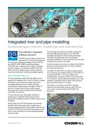
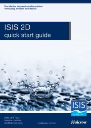
Cost effective, integrated modelling solutionsThink saving, think ISIS, think HalcrowISISquick start guide0845 094 7994halcrow.com/isisisis@halcrow.comA CH2M HILL COMPANYby HalcrowTECHNOLOGYTechnology

ISISQuick Start GuideOverviewThis quick start guide enables first time users to quickly understand how to use ISIS to construct andrun simple river models. The guide explains some of the basic concepts of ISIS model constructionand the various files used to run a model, also included is a step-by-step guide for constructing asimple river model:• Chapter 1 “Starting ISIS and Basic Concepts” explains how to start your ISIS software andgoes through some basic concepts.• Chapter 2 “How to Run an Existing Model” shows an example of running an already preparedmodel, in this case it is a model of a tidal river.• Chapters 3, 4 and 5 illustrates the principles of building common elements of river models,such as a single channel, a simple network and adding weirs.• Chapter 6 “How to Run a Flow Model” focuses on the steps needed for running a flow model.This chapter contains a more general explanation of model running than that provided inChapter 2.• Chapter 7 “How to View Simulation Results” describes the steps needed for the visualisationof the results of the ISIS simulation.Table of Contents1. Starting ISIS and Basic Concepts ...................................................................................................... 32. How to Run an Existing Model ........................................................................................................... 43. How to Build a Single Channel......................................................................................................... 114. How to Build a Simple Network ........................................................................................................ 155. How to Add Weirs to the River Model .............................................................................................. 186. How to Run a Flow Model ................................................................................................................ 207. How to View the Simulation Results................................................................................................. 238. Further Information ........................................................................................................................... 27Do you have any questions or remarks? Please contact ISIS support at isis@halcrow.comor on 0845 094 7994 (+44 1793 845733 from outside the UK) www.halcrow.com/isis2

ISISQuick Start Guide1. Starting ISIS and Basic ConceptsStarting ISISOnce you have installed the software and rebooted your PC you will be ready to use ISIS. For ISISProfessional users you may need to copy the ISIS licence file (isis.set) into the ISIS folder (egc:\isis\bin) and attach the hardware key or dongle. Then, from the Start menu, select Programs, thenselect the ISIS group and click on the ISIS icon . If you are using the Network Licence please followthe instructions in the documentation provided with your licence file. If you have any questions pleasedo not hesitate to contact ISIS support (details are at the foot of this page).The main user interface of ISIS is the Network Properties Window, which opens automatically everytime ISIS is launched. The Network Properties Window is used to enter and view the details of modelcomponents such as river channels and weirs, the initial and boundary conditions and the connectivityof the hydraulic units that make up the model.Basic ConceptsISIS can be used to model flows and water levels in open channels and floodplains. A wide range ofstructures, including bridges, sluices, culverts, pumps and weirs can also be modelled.An ISIS model is constructed using a number of different hydraulic units, which can be thought of asbuilding blocks that are connected together. In most cases, an ISIS model must have the followingthree types of unit as a minimum:• Upstream boundary: to represent the flow entering the model.• Downstream boundary: to represent the downstream water level.• At least 2 river/routing/conduit sections: to represent the river channel.Each unit contains model data appropriate to the unit type, e.g. a River Section unit contains crosssectiongeometry and roughness data for the river. Units also contain one or more node labels in orderto be able to identify the unit and to be able to define the connectivity with other units in the model.Units with the same label are automatically connected. River Section and Conduit units are connectedtogether in the order in which they appear within the Network Properties Window, from the beginningto the end of the particular channel reach (the end of a river reach is signified by a zero distance stepin the last River Section unit).Note that in this quick start guide we use the shorthand > Name to mean click on the menu item called‘name’, for example ‘> File > Open’ means click on the menu item File then click on submenu itemOpen.Do you have any questions or remarks? Please contact ISIS support at isis@halcrow.comor on 0845 094 7994 (+44 1793 845733 from outside the UK) www.halcrow.com/isis3

ISISQuick Start Guide2. How to Run an Existing ModelThe Chapter shows an example of running a model simulation using the model that has already beenprepared. There is a number of existing examples placed onto the “isis” folder of your machine duringthe installation of ISIS. The default location for your “isis” is C:\isis\data (if ISIS is installed at a locationother than the default folder, it will be xxx\xxx\isis\data where xxx stands for where ISIS is installed).This Chapter will explain how to access the ISIS sample file, interpret what it represents, show theway we can run the simulation based on this file and will help you go through the results obtainedduring this simulation.1) Launch ISIS. The ISIS user interface is shown on Figure 1.Figure 1. ISIS user interface2) Open an example file > File > Open or click the open icon , then browse to the isis\data folder,open the file called “TIDAL.DAT”. Click “No” when it asks you to load the water quality data (here weare just going to run a flow model without a water quality component - please note ISIS Free cannotoperate with the water quality). After loading the tidal model the ISIS user interface should look likethat shown on Figure 2.Do you have any questions or remarks? Please contact ISIS support at isis@halcrow.comor on 0845 094 7994 (+44 1793 845733 from outside the UK) www.halcrow.com/isis4

ISISQuick Start GuideFigure 2. The model contained in tidal.dat file shown in ISIS Network Properties windowThis is a model for a river with a strong tidal influence. Before the simulation is run, let’s view themodel of the river in the Visualiser and look at the representation of the boundary conditions.3) View the river model in the Visualiser. To do this, click the Visualiser icon or select > Tools >Visualiser from the main menu, click ‘Ok’ when the coordinate dialogue appears on the screen. NowFigure 3 shows the representation of the model contained in the file TIDAL.DAT in the Visualiser. Theuser can see that the river in this model is a straight single channel.ISIS actually contains three options for plan views of the model:• Visualiser - for simple schematic views of the model• GIS Visualiser - this can show either a schematic view or a 2D ‘real world’ GIS view withraster and vector data as background images• ISIS Mapper - for 2D and 3D ‘real world’ GIS views of selected ISIS data along with rasterand vector data. ISIS Mapper also includes functions for model building and flood mapping.Do you have any questions or remarks? Please contact ISIS support at isis@halcrow.comor on 0845 094 7994 (+44 1793 845733 from outside the UK) www.halcrow.com/isis5

ISISQuick Start GuideFigure 3. The model contained in a sample file TIDAL.dat shown in the Visualiser Tool of ISIS4) View the longitudinal profile of the channel. To do this, close the Visualiser and go back to the mainISIS user interface. Select all the river section units by first selecting the first unit in the model (node2.1) and then scroll down to the end of the model (label 3.38) and press the key together withthe left mouse button. Then, right mouse click the selected sections and choose ‘Long Section’ (oruse short cut key or click the long section picture icon ). Select Plot to generate thegraph.The long section profile that you should see at this stage is shown on Figure 4 (if the blue area ismissing then this indicates that model results are not yet available – we will be generating results laterin this section). This picture clearly shows the varied bed profile as well as the water level rising to theleft of the screen. You can see that most of the water in this figure is actually below the sea level(shown by the mark 0 on elevation scale in the left-hand side of the graph).Figure 4. The plot of the longitudinal profile of the river represented by the model in TIDAL.DAT fileDo you have any questions or remarks? Please contact ISIS support at isis@halcrow.comor on 0845 094 7994 (+44 1793 845733 from outside the UK) www.halcrow.com/isis6

ISISQuick Start Guide5) View the downstream boundary condition. Go back to the main ISIS user interface of the tidalmodel shown on Figure 2. Double click the HTBDY unit 3.38 (HTBDY is the ISIS shorthand for HeadTime BounDarY). Click the ‘Plot’ button of the dialogue that appears. It will show you the plot of thewater level–time series of the downstream boundary condition of the model in the TIDAL.DAT file. Thisplot is shown on Figure 5. You can see that the downstream boundary condition for this model is of atidal nature.Figure 5. Plot of the downstream boundary condition of the model in the TIDAL.DAT fileshowing a typical tidal time seriesWe can also view the upstream boundary condition using the same procedure, but choosing theupstream boundary condition node (2.1) – you will have to close the HTBDY data form first by clickingon its Cancel button. This boundary condition is represented by a constant flow of 100m 3 /s.6) View one of the cross sections. Double click one of the river section units (for example section2.12), click the ‘plot’ button of the dialogue that appears on the screen, then you should see the graphof a cross section on the screen. In the right hand side of the plot you can see the cross-sectionalprofile of the river with a flood wall on the right hand side and to the left of the river you can see a floodplain (250 m wide) with a steep hill on the left-hand side. Cancel the view of the cross section data.Do you have any questions or remarks? Please contact ISIS support at isis@halcrow.comor on 0845 094 7994 (+44 1793 845733 from outside the UK) www.halcrow.com/isis7

ISISQuick Start GuideFigure 6. Profile of the cross section 2.12 of the model in the TIDAL.DAT file7) Run the simulation. Click the ‘flow simulation’ icon or select > Run > Flow simulation. A flowsimulation run form interface will appear as shown by Figure 7.Figure 7. The interface for running the model in the TIDAL.DAT fileSelect the Unsteady (Fixed Timestep) button, set the “Finish time” to 36 hours and set both the“Timestep” and “Save interval” to 360 seconds. Click Run. Click “Exit” after the simulation completes(see Figure 8) and “Close” the run model scenario dialog without saving Scenario data (Figure 7).Do you have any questions or remarks? Please contact ISIS support at isis@halcrow.comor on 0845 094 7994 (+44 1793 845733 from outside the UK) www.halcrow.com/isis8

ISISQuick Start GuideFigure 8. The ISIS window showing the completion of unsteady simulation runof the model in the TIDAL.DAT file8) View the results. First let’s view the water level time series at one of the river sections. It should bea tide graph similar (but not identical) to the one of the downstream boundary condition shown byFigure 5. To do this, right click one of the river sections (for example section 2.26) and select timeseries and click ‘Plot’. The water level result at this section will be plotted. It is shown by Figure 9.Figure 9. Time series plot for one of the river sections of the model in the TIDAL.DAT fileUsing the ability of ISIS to animate the results we can watch a dynamic animation of the changes ofthe water level with time on the longitudinal profile of the river. To do this we have to plot the longsection of the river (the way to plot this are explained in step 4 of this Chapter), right mouse clickinside the long section and click ‘animation’, then click the “Play” button ( )on the animation toolbarat the top of the screen. The simulation results of the model in TIDAL.DAT will be animated.Figures 10 to 14 illustrate the changes of the water level in the river represented in the file TIDAL.DATin the course of the simulation described earlier. You can see that the changes of the tidal cycle alongthe river.Do you have any questions or remarks? Please contact ISIS support at isis@halcrow.comor on 0845 094 7994 (+44 1793 845733 from outside the UK) www.halcrow.com/isis9

ISISQuick Start GuideFigure 10. Water level at T=0hFigure 11. Water level at T=3hFigure 12. Water level at T=6hFigure 13. Water level at T=9hFigure 14. Water level at T=12hDo you have any questions or remarks? Please contact ISIS support at isis@halcrow.comor on 0845 094 7994 (+44 1793 845733 from outside the UK) www.halcrow.com/isis10

ISISQuick Start Guide3. How to Build a Single ChannelThis Chapter explains the ways of building a model representing a single channel, i.e. a reach of riverthat is not branched.A single channel contains at least four units: upstream boundary condition, downstream boundarycondition and two sections to represent a channel. Figure 15 shows a very simple channel with eightcross sections.QTBDY is shorthand for the discharge (Q) Time series BounDarY condition (for the upstream inflow tothe channel). HTBDY represents the water level time series boundary condition for the downstreamend of the channel.QTBDYHTBDYFigure 15. A schematic representation of a single channel with eight sections andtwo boundary conditionsIn order to build such a channel, we have to follow the following steps:1. Start a new (blank) model in ISIS (> File > New)2. Insert a Flow-Time Boundary (QTBDY) unit to represent an upstream boundary. To insert this unityou can either click on the Flow-Time Boundary picture button or select > Edit > Insert >Boundaries > Hydrographs > Flow/Time from the main menu. When the Node label editor dialogappears, enter the label S1 (in upper case), and click ‘OK’. Save this file with a proper name (forexample, singleChannel.DAT) and choose the location on your computer to place a copy of the file.3. Specify the data for the boundary condition. Double click on the newly inserted unit to display thedata entry screen for the boundary. Enter the flow data into the Flow-Time table. As shown by theexample below: let’s enter a simple hydrograph, peak flow 20m3/s, base flow 10 m3/s and time topeak is 12 hours. Remember to make sure that the unit of the time is hours (by default it is “seconds”).Do you have any questions or remarks? Please contact ISIS support at isis@halcrow.comor on 0845 094 7994 (+44 1793 845733 from outside the UK) www.halcrow.com/isis11

ISISQuick Start GuideFigure 16. Flow-Time data entry form.4. Insert a River Section unit. To insert this unit you can either click on the River Section picture buttonor select > Edit > Insert > Channels > River > River Section from the main menu. When theNode label editor dialog appears, enter the label S1 (in upper case) and click OK.Figure 17. Connection of a river unit to a QTBDY unit5. Click 'Yes' when asked whether you would like to connect the S1 labels. This River Section unit islocated immediately downstream of the Flow-Time Boundary (hence the node labels of these units arethe same).6. Enter the cross section data. Double click on the newly inserted unit to display the data entry screenfor the River Section. Enter the cross section data into the table, leaving the rest of the parameters inthe table at their default values:Do you have any questions or remarks? Please contact ISIS support at isis@halcrow.comor on 0845 094 7994 (+44 1793 845733 from outside the UK) www.halcrow.com/isis12

ISISQuick Start GuideFigure 18. Specification of the cross section data7. View the cross-sectional profile of the cross-section by clicking on the Plot button. In this simpleexample we have used a triangular cross section.Figure 19. Plot of the cross section profile8. Specify the distance between the cross-sections. Enter a certain value for the 'distance to nextsection' field, for example 100 metres.9. Specify the cross-section data for all the cross-sections. Repeat the same procedures 8 times toinsert 8 river sections, name them S1 to S8 (to save time you can use copy and paste).Note that: the last section must have a ‘distance to next section=0’, this is used by ISIS to recognise itas the last section of a channel reach.10. Specify the information for the downstream boundary condition. For the last channel section aHTBDY boundary condition unit is inserted in a similar manner as the first QTBDY boundary conditionunit (by clicking the picture icon , and prescribing the time series data in the table, for example aconstant water level of 2 meters).Do you have any questions or remarks? Please contact ISIS support at isis@halcrow.comor on 0845 094 7994 (+44 1793 845733 from outside the UK) www.halcrow.com/isis13

ISISQuick Start GuideFigure 20. The Stage-Time data entry form for the downstream boundary condition S8.11. Visualise the river model. After building the single channel, we can use Visualiser to visualise thechannel that we have just been build. This is done by clicking on the Visualiser picture icon or select> Tools > Visualiser from the main menu.Note: Please remember to save your file. For the information on how to run a simulation and view theresults please refer to other sections of this quick start guide.Do you have any questions or remarks? Please contact ISIS support at isis@halcrow.comor on 0845 094 7994 (+44 1793 845733 from outside the UK) www.halcrow.com/isis14

ISISQuick Start Guide4. How to Build a Simple NetworkThis Chapter describes the way of building a model of a branched river (i.e. a river network). Theexample river network consists of a main channel and tributary channel (Figure 21).S4UpJunctionS4DnT4Figure 21. A schematic representation of a simple network.For the main channel, S1, S2…S8 are the labels for its cross-sections. T1, T2, T3 and T4 are thelabels for the tributary channel.As shown in Figure 21, a junction should be built to link the main channel and the tributary at sectionS4. In order to insert a junction at section 4, we have to split section S4 into two sections: S4Up andS4Dn. Then we should place the junction in between S4Up and S4Dn. Please note that we specify thefield “distance to next section” for S4up section as 0, which physically means S4Up and S4Dn are thesame section.The detailed procedures of building a simple network are described below:1. Start ISIS and begin a new model.2. Build the upstream boundary condition unit (by clicking on one of the icons of the Boundaries Toolbar eg QTBDY boundary icon ). It should be built in the same manner as described in Chapter 3.Here we will name this QT boundary as S1. Save the file with the name simpleNet.DAT.3. Specify the hydrograph for the upstream boundary condition unit. Double click on the QTBDY unitin the Network Properties window in ISIS. Enter the time series in the QTBDY boundary table thatopens, for example, take the same hydrograph as described in the Step 2 of Chapter 3.Figure 22. Flow-Time boundary data entry form for the upstream boundary conditionDo you have any questions or remarks? Please contact ISIS support at isis@halcrow.comor on 0845 094 7994 (+44 1793 845733 from outside the UK) www.halcrow.com/isis15

ISISQuick Start Guide5. Build the first cross-section S1. You can do this by clicking the River Section picture icon ; enterinput cross section data in the table that opens on the screen.Figure 23. Cross-section data entry form6. Build sections S2, S3, and S4Up in the same manner as for S1, please note that the S4Up shouldalso have the “distance to next section” field set to 0, which means S4Up and S4Dn are samelocation.7. Build the Junction and connect this junction to sections S4Up, S4Dn and T4 (S4Dn and T4 will bebuilt later on). To do this, either click the Junction unit icon or select > Edit > Insert and then >Junction > Open JunctionFigure 24. Connecting the river units to a junction unit using the Node label editor form8. Build sections S4Dn, S5 to S8 (cross section shapes can be the same or different).Do you have any questions or remarks? Please contact ISIS support at isis@halcrow.comor on 0845 094 7994 (+44 1793 845733 from outside the UK) www.halcrow.com/isis16

ISISQuick Start Guide9. Build downstream boundary condition (say HTBDY) for the main channel S8 and link it to sectionS8. The stage-time boundary can be a constant of 2 metres.10. Build tributary sections T1, T2, T3 and T4.11. Build the upstream boundary condition (QTBDY) for the tributary T1 and link it to the section T1(by having the same label).Note: Remember that the last section of each branch (ie T4) has the ‘distance to next section=0’Figure 25 shows the completed model.Figure 25. The completed simple river network model.Note: Do not forget to save your file again after building everything. For running the simulation pleaserefer to Chapter 6 of this quick start guide.Do you have any questions or remarks? Please contact ISIS support at isis@halcrow.comor on 0845 094 7994 (+44 1793 845733 from outside the UK) www.halcrow.com/isis17

ISISQuick Start Guide5. How to Add Weirs to the River ModelThis Chapter describes the way a user can model hydraulic structures such as weirs in ISIS.ISIS can deal with various types of hydraulic structures; the general weir unit is one of the most oftenused structures.The Figure 26 shows a simple channel with a weir built in:ChannelCross sectionWeirFigure 26. A schematic representation of a weir built into a river modelFigure 27 (Along the right hand side of the page). Visualisation of the channel with theweir between sections S3 and S5.In order to place a weir in an existing modelled reach, we first split our river reach intotwo (ending the first reach with a ‘distance to next section=0’) and place the weir betweenthe two sub-reaches. The figure on the right illustrates how this can be done in ISIS:Detailed procedures to build a weir in the channel are covered below:1. Start ISIS and start a new model (or copy an existing single reach model and adjustthe following instructions to suit).2. Build an upstream boundary condition unit, for example a flow-time unit S1 (seeChapter 2). Save the model file as the name Weir.dat.3. Prescribe the time series in the QT boundary table in the same manner as described in Steps 2 ofChapters 2 and 3 of this guide.4. Build the first river section S1 and connect it to the boundary unit S1 we have just built (asdescribed in steps 4 and 5 of the Chapter 3).5. Build sections S2, S3, and S4Up in the same manner as described in Step 9 of the Chapter 3.Please note that the S4Up has the field “distance to next section” set to 0, which means S4Up andS4Dn are same section.7. Build the weir after section S4Up and input the upstream label as S4Up and downstream labelS4Dn. To do this, either click the general purpose weir icon or select > Edit > Insert then >Structures > Weirs > Weir.Do you have any questions or remarks? Please contact ISIS support at isis@halcrow.comor on 0845 094 7994 (+44 1793 845733 from outside the UK) www.halcrow.com/isis18

ISISQuick Start GuideFigure 28. Connection of the weir unit to the river model using the Node label editorFor the configuration of the weir parameters you should specify the elevation of the crest and thebreadth of the crest. Other parameters can be left with the default values. To do this, double click theweir unit and the Figure 29 will appear on the screen.Figure 29. Entry form for the parameters of the unit Weir8. Build sections S4Dn, S5 to S8 (cross section shapes can be same or different) as in Chapter 3.9. Build the downstream boundary condition (for example HTBDY) for the main channel S8 and link itto section S8 (as in Chapter 3).Do you have any questions or remarks? Please contact ISIS support at isis@halcrow.comor on 0845 094 7994 (+44 1793 845733 from outside the UK) www.halcrow.com/isis19

ISISQuick Start Guide6. How to Run a Flow ModelThis Chapter describes how to run of an ISIS model. Some details of running a flow model were givenin Chapter 2; this Chapter provides more information.To run a simulation in ISIS you should follow the steps below:1. Start ISIS2. Load the model. As an example we can load the simple channel model we built in the Chapter 3 ofthis guide. Select > File > Open and browse to the folder that contains the .dat file (ISIS model file),select it and click Open.Note: before starting the simulation, all the boundary condition data and cross section shape datamust be prescribed. For this example, we can use the following information. It is a straight rectangularchannel with a length of 700 metres. The shapes of the cross sections, upstream QTBDY anddownstream HTBDY are shown in Figure 30.Figure 30. Key model data (from left to right): downstream boundary condition; upstream boundarycondition and cross section data3. Click the ‘Flow simulation’ icon or select > Run > Flow simulation. A flow simulation run forminterface will appear. It is shown on the Figure 31.Figure 31. Run form interfaceDo you have any questions or remarks? Please contact ISIS support at isis@halcrow.comor on 0845 094 7994 (+44 1793 845733 from outside the UK) www.halcrow.com/isis20

ISISQuick Start GuideIn this example we will only deal with the ‘Times’ tab which has a button named ‘Run’ on the bottomleft side. Detailed information about the tabs and buttons of this form can be found at > Help >Contents > Using ISIS > ISIS user interface > Run Forms Interface.There are five simulation types displaying on the ‘Times’ tab. For this simple river channel model, the‘Steady (Direct)’ and the ‘Unsteady (Fixed Timestep)’ options are used. These two types are explainedin more detail below.It is highly recommended to run a steady simulation before the unsteady one.4. Running a steady simulation. Select ‘Steady (Direct)’ simulation type and click on the ‘Run’ button(or go to Run > Flow simulation in the ISIS run Scenario screen).After that a window will appear on the screen, which will show the progress of the simulation. After thesimulation finishes, a message ”simulation completed” will appear. After that you can view the steadysimulation results by clicking the ‘View’ button. If there are errors during the simulation, the processwill stop and an error message will be shown.For more on viewing the results please refer to the Chapter 7 “How to View Simulation Results” of thisguide.Figure 32. Notification of the successful completion of a simulation5. Running an unsteady simulation. Select ‘Unsteady (Fixed Timestep)’ simulation type. Enter the‘start time’ and ‘finish time’. The time span for simulation must be within the range of the shortesttime span of the boundary conditions which are defined in the model set-up step. Also, the time stepand save interval should be defined (for example 10s for time step and 60 s for save interval).6. Click on the ‘Run’ button (or go to Run > Flow simulation) after prescribing the parameters for theunsteady simulation. A window will pop up showing the simulation process and some important figuresfor the model (see Figure 33).Do you have any questions or remarks? Please contact ISIS support at isis@halcrow.comor on 0845 094 7994 (+44 1793 845733 from outside the UK) www.halcrow.com/isis21

ISISQuick Start GuideFigure 33. The progress of the unsteady simulation in ISIS7. After finishing the unsteady simulation, the summary outputs can be viewed in the form of plain text.However, other methods for visualisation of the model results can be used. Please see Chapter 7 ofthis guide.Do you have any questions or remarks? Please contact ISIS support at isis@halcrow.comor on 0845 094 7994 (+44 1793 845733 from outside the UK) www.halcrow.com/isis22

ISISQuick Start Guide7. How to View the Simulation ResultsThis Chapter describes how to view the ISIS model results generated from a simulation.Normally both steady and unsteady simulation results are stored in the same folder that the model hasbeen stored in. Following the example used in Chapter 3, it will be the single channel model.The steady simulation results are stored in an ASCII file which has an extension of .zzs. Please notethat this file can be viewed and modified in a normal ASCII editor like Notepad, WordPad, etc.In order to view the steady simulation results, you can browse to the folder where you stored yourmodel. Figure 34 shows an example of a .zzs opened using the WordPad.Figure 34. An example of a .zzs steady results file opened in WordpadIn this file flow (m 3 /s), stage (m elevation) and other information such as Froude number and velocityare recorded for each channel section.The unsteady results are stored in a binary file which has an extension of .zzn. This file cannot beopened in an ASCII editor and we must use ISIS to view the results.The following options are available for viewing the results – the first three are described in this guide:• Time series plot in the form of water levels and discharges at each section.• Long section profile of the water levels• Animations of the long section profiles of the water levels• Cross sections with water levels displayed• X-Y plots, eg rating curves• Tabulated results generated from the ISIS TabularCSV tool• 2D and 3D flood maps created in ISIS MapperViewing the ISIS simulation results by means of plotting the time series1. Start ISIS2. Load the models for which you have the results of the unsteady simulation run. Select > File >Open and browse to the folder that your model files are stored in.3. Right click the section for which you would like to plot the time series and select ‘Time series’ (orselect the section and use the short cut key).Do you have any questions or remarks? Please contact ISIS support at isis@halcrow.comor on 0845 094 7994 (+44 1793 845733 from outside the UK) www.halcrow.com/isis23

ISISQuick Start GuideFigure 39. Animation of a long section water level profileFor more information about the Graphical Output and animations please refer to the ISIS help file inthe section Using ISIS > Graphical Output.Do you have any questions or remarks? Please contact ISIS support at isis@halcrow.comor on 0845 094 7994 (+44 1793 845733 from outside the UK) www.halcrow.com/isis26

ISISQuick Start Guide8. Further InformationA full description of the capabilities of ISIS is provided in the online help system accessed from the >Help > Contents menu item. In addition Halcrow provides training courses to help you get the mostout of ISIS – for further details of training courses please refer to www.halcrow.com/isis.This quick start guide should have provided you with an introduction to how to use ISIS. The ISISsoftware system is a complex simulation and visualisation package which has many options andfeatures not discussed in this guide. For example, starting with version v3.0, ISIS includes the ISISMapper component that allows 2D and 3D visualisation, automated generation of input files andproduction of flood maps. It can be accessed by clicking the ISIS Mapper icon or selecting > Tools> ISIS Mapper. For more information on how to use ISIS Mapper, refer to the ISIS Mapper section ofthe help file (> Help > Contents > ISIS Mapper).Do you have any questions or remarks? Please contact ISIS support at isis@halcrow.comor on 0845 094 7994 (+44 1793 845733 from outside the UK) www.halcrow.com/isis27