Paper - Caris

An integrated approach to acquiring sound speed proles usingthe Regional Ocean Modeling System (ROMS) and anAutonomous Underwater Vehicle (AUV)Gretchen Imahori, Lyon Lanerolle, Steven Brodet,Robert Downs, Jiangtao Xu, Ruby Becker, and Lorraine RobidouxSeptember 16, 2008AbstractWith the inception of Multibeam Echosounder Systems (MBES) and the use of the CombinedUncertainty and Bathymetry Estimator (CUBE) algorithm, determining sound speed prole locationsand sampling frequency a priori is necessary to eectively model the sound speed component of theTotal Propagated Uncertainty (TPU) of echosounder depths. Currently, sound speed sensors are notused in the most eective manner, causing oversampling in some areas and undersampling in others.This can cause undue `wear and tear' on a sensor when it is used in a near continual manner and/orcan cause sound speed induced refraction errors due to insucient samplings applied to multibeamdepths. In this paper, we describe a case study to show proof-of-concept in which we use RutgersUniversity's Regional Ocean Modeling System (ROMS) to help us identify a priori sound speedcast locations and an Autonomous Underwater Vehicle (AUV) tted with a CTD sensor to acquirecomponents to calculate sound speed data in the vicinity of Solomons, MD. In return, the salinityand temperature observations acquired via the CTD will help to validate the physical oceanographysimulated by the model. It is hoped that this eort will benet the hydrographic community indetermining where to eectively sample sound speed and in accessing the environmental uncertaintycomponent which is often the largest contributor to sound speed uncertainty.1 IntroductionFrom the advent of acoustic depth sounding systems the dependance upon sound speed information hasbeen known; however there has been renewed interest with the development of Multibeam EchosounderSystems (MBES) and the use of the Combined Uncertainty and Bathymetry Estimator (CUBE) algorithm.One of the main causes for MBES depth measurement errors is often `sound speed errors'.However, it is not necessarily the sound speed measurement that is in error, but often that the wrongsound speed prole was applied to the data. Taking an insucient number of sound speed casts, thusignoring the spatio-temporal variability of the ocean, typically results in the user applying an sound speedprole that is not indicative of the area, thereby biasing the depth and position of a MBES sounding.CUBE allows the sound speed component of the Total Propagated Uncertainty (TPU) to be modeledmore eectively. If a biased sound speed component is entered into the uncertainty model, the ability ofthe algorithm to distinguish deleterious eects of refraction may be reduced. Therefore, determining thesound speed prole locations and sampling frequency a priori is necessary to reduce the `sound speed1

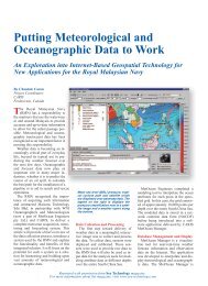
errors' and eectively model the sound speed component of the TPU of MBES depths (Imahori, 2007).Currently, sound speed sensors are not used in the most eective manner, causing oversampling in someareas and under sampling in others. The present method to resolve the lack of sampling is to acquiresound speed data in a near continual manner (e.g. using a moving vessel proler with a sound speedsensor) when possible. While this method has proved to be adequate in many cases, it will undoubtablyshorten the sensor equipment operational lifetime.To test a new approach, on May 28 and July 8-9, 2008 in Solomons, MD, we used a Hydroid REMUS100 Autonomous Underwater Vehicle (AUV) tted with a SBE 49 FastCAT CTD sensor (Figure 1) toacquire temperature, salinty and pressure data (which would be used to calculate sound speed and thuscreate sound speed proles (SSP)).Figure 1: Image of the REMUS 100 AUV tted with SBE 49 FastCAT CTD sensor being deployed.The purpose of this experiment was to create a proof-of-concept method using the REMUS to completelycharaterize sound speed uncertainty in a hydrographic project area. Moreover, the ship couldcontinue acquiring multibeam data while the REMUS acquired data for calculating sound speed. Eachposition of the AUV dive (and therefore sound speed cast location) taken July 8-9 was determined withthe aid of the Rutgers University's Regional Ocean Modeling System (ROMS) for the Chesapeake Bay.While NOAA's Coast Survey Development Lab (CSDL) has been working with the REMUS AUV andthe ROMS for a few years, this is the rst time that the two have been used in tandem. This paper hopesto lay the ground work for using the ROMS, when it is available, to support NOAA's use of an AUV toacquire SSPs in the most ecient manner. The ROMS model application domain covers the whole of theChesapeake Bay, from the entrance of the Sasquehanna River in the north to the 100m isobath on theshelf in the south and Washington, DC in the west to Ocean City, MD. The model bottom bathymetrywas created from inverse-square interpolation of National Ocean Service (NOS) sounding measurements.In this paper we will discuss the specications of the REMUS and the ROMS, how the ROMS particlepath tracking was utilized to determine sound speed cast locations and the preparation involved withusing both the REMUS and ROMS. Additionally, this paper will describe the two experiments to enhanceour understanding of how to run the AUV in a cast mode senario and to collect sound speed proles to test2

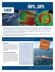
and rene our algorithm which would be then inserted into NOAA's Velocwin software. Finally, we willdiscuss our results of our rened algorithm and how we conducted a temperature and salinity validationexercise. This proof-of-concept experiment will not only be a benet to hydrographers by helping themdetermine where to eectively sample sound speed and access the environmental uncertainty componentof sound speed (Imahori and Hiebert, 2008), but it will also help NOAA validate the ROMS with thesalinity and temperature observational data collected by the REMUS.2 ProjectNOAA's Oce of Coast Survey maintains the Survey Vessel BAY HYDROGRAPHER (Figure 2), whichis homeported in Solomons, MD. The vessel serves as the primary test and evaluation platform for CSDL.Initial plans were to deploy the REMUS with the FastCAT CTD sensor from the Bay Hydrographer todevelop mission planning guidelines in the familiar environment of the Chesapeake prior to conductingoperational testing in the dynamic and harsh environment of Kachemak Bay, Alaska for NOAA'sHydropalooza (http://oceanservice.noaa.gov/hydropalooza).Figure 2: NOAA S/V BAY HYDROGRAPHERDuring the planning of this project and discussions of future work on sound speed with CSDL (Imahoriand Hiebert, 2008), a ROMS application to the Chesapeake Bay (CBOFS2 - Chesapeake Bay OperationalForecast System which is currently under development) was brought to our attention. It was hoped thatthis model set-up would allow us to gain an understanding of the physical oceanography of the Solomonsregion and provide guidance as to where we should acquire CTD (thus SSPs) with the REMUS.Unlike the salinity and temperature data we were planning on using from the BAY HYDROGRA-PHER's past projects to deduce the oceanographic variability, the ROMS via Lagrangian particle pathtracking, would enable us to see the eects the tidal water elevations and currents thus showing the movementsof the water 'parcels' both in the horizontal and the vertical (up and down the water column).This would in turn provide us with added information about the extent of the horizontal and verticalmixing/dispersion associated with the intervals of the tidal cycle for our SSP collection.The REMUS 100 AUV weighs approximately 55 kg and is 180 cm in length. The REMUS can operateat a maximum depth of 100 m and has an endurance of up to 18 hours. The REMUS's maximum speedis 5 knots, but typical survey speed is 3-4 knots. The REMUS can not work eectively in areas wherethe current is greater than 3 knots.3

The REMUS 100 primarily uses a GPS-aided Inertial Navigation System (INS) for positioning andnavigation, but can also operate with a Long Baseline (LBL) acoustic transponder system. The navigationsystem initializes the REMUS's position on the surface using WAAS enabled GPS. This AUV candetermine when the navigation solution needs an updated GPS x automatically, but the user can denethe maximum time between xes, program a forced x, or force dead reckoning (we typically let the AUVdetermine when it needs a x, but set the max time between xes to 30 minutes). Once submerged,the vehicles position is calculated using the Kearfott INS coupled speed over ground information derivedfrom an RDI Instruments Acoustic Doppler Current Proler (ADCP). The REMUS will alter its depthto avoid collision if it detects a rise in the seaoor; however, it does not have a forward-looking collisionavoidance capability, so care must be taken during mission planning when the operating area is likely tocontain obstructions, such as shing traps or kelp.During operations the operators can communicate with the REMUS via acoustic modem deployedeither from the vessel or a Gateway buoy, which includes a radio modem to relay data between the buoyand base station on the vessel.The SBE 49 FastCAT CTD sensor on the AUV acquires conductivity (which is used to calculatesalinity), temperature, and pressure data. The REMUS operating system collects the SBE 49 data andoutputs a text le with position, time, salinity, temperature, depth, and sound speed.2.1 Preparation work2.1.1 ROMSROMS is a split-explicit, nite dierence based orthogonal, curvilinear grid numerical ocean model(Shchepetkin and McWilliams, 2004). The vertical grid is based on a stretched terrain-following sigmacoordinate system (Song and Haidvogel, 1994). Both the momentum and tracer advection terms are discretizedusing high resolution, third order upstream-biased advection schemes which alleviate the need toadd explicit horizontal viscosity/diusivity in the numerical computations(Shchepetkin and McWilliams,1998). The hydrostatic pressure gradient terms are also discretized using an extremely robust and accuratepiecewise cubic spline construction (Shchepetkin and McWilliams, 2003). The vertical turbulence/eddymixing is carried out using a standard Mellor-Yamada 2.5 scheme (Mellor and Yamada, 1982), a KPPscheme, or a family of General Length Scale (GLS) schemes consisting of k-epsilon, k-tau and k-omegaschemes(Warner et al., 2005). A perfect restart formulation in the ROMS allows lengthy computationsto be carried out as a sequence of smaller segments. Along the ocean bottom bathymetry, friction canbe prescribed with a logarithmic, linear, quadratic law, or a Bottom Boundary Layer (BBL) formulation(Styles and Glenn, 2000). At the ocean surface, the surface meteorological forcing can be imposed intwo ways in ROMS (a) if the wind stresses and net heat uxes are available, they can be prescribeddirectly, but otherwise, (b) the wind speeds, air pressure, air temperature, relative humidity, net shortwaveradiation and downward longwave observations when available could be fed into ROMS and thewind stresses and the net heat ux can be estimated internally via a Bulk Flux formulation (Liu et al.,1979). If downward longwave radiation data is unavailable, the net longwave radiation can be computedinternally using the Berliand formulation (Berliand and Berliand, 1952). Cloud cover and precipitationmay also be included in the calculations but they were not employed in the work associated in this article.The computational domain extended from Washington, DC in the West to Ocean City, MD and fromthe 100m isobath on the shelf in the South to the Susquehanna river in the North. The curvilinear,orthogonal grid for the Chesapeake Bay was generated via the DELFT3D grid generator (Delft3D, 2008).The model bottom bathymetry was formed by inverse-square interpolation of the NOS soundings measurements.There were 291 x 332 grid points in the horizontal (resolution : 34m ≤ Δx ≤ 4895m and 29m4

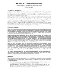
≤ Δy ≤ 3380m in the two spatial directions) and 20 vertical sigma levels. A plot of the grid is given inFigure 3.Figure 3: Image of ROMS gridThe initial conditions were formed by interpolating the temperature and salinity elds from the WorldOcean Atlas (WOA) 2001 (Conkright et al., 2002) on to the ROMS model grid (and thereafter spinningup from rest).As for the model forcings: (i) the river forcings were created out of United Stated Geological Survey(USGS) river discharge data and the river temperature and salinity were obtained from Maryland Departmentof Natural Resources (MD-DNR) and the Chesapeake Bay Program; (ii) along southern openocean boundary, the tidal water level predictions from the ADCIRC tidal harmonics database (Luettichet al., 1992) were combined with the non-tidal components extracted from the water levels at Duck, NC,Ocean City Inlet, MD (NOAA Center for Operational Oceanographic Products and Services (CO-OPS)tide gauges). The temperature and salinity along this boundary were interpolated from the WOA 2001climatology.; (iii) the meteorological forcings consisting of the two wind speed components, air pressure,temperature, relative humidity, downward longwave radiation ux and the net shortwave radiation uxwere all obtained from the North American Mesoscale (NAM) 12 km resolution model 3-hourly forecasts.The wind stresses and the net heat ux were computed within ROMS via the bulk ux parameterization.The model simulation was carried out from April 15, 2008 to July 15, 2008 thereby allowing a sucient5

duration of time for the ow-elds to evolve. The river discharges, tidal water levels and the winds wereramped-up over a 5-day period to enable stable and smooth spin-up (from rest). A quadratic bottomfriction formulation was employed with a drag coecient of 0.005 throughout the model domain. Thebaroclinic time step employed in the computations was 30 seconds.For the particle tracking phase of the simulations, a simplied set-up was sucient, and hence employed,and it involved using constant temperature and salinity throughout the computations with theonly model forcing being provided by tides which is the main driving force behind the movements ofthe water column. The tidal forcing did not include the sub-tidal component which is usually not assignicant as the purely tidal component. This simulation was from June 27, 2008 to July 09, 2008. Thecurrents used for the particle tracking were those of July 08 and July 09 by which time the tidal ow hadfully developed. The particle tracker employed was one developed within CSDL which has a second-orderRunge-Kutta time stepping algorithm. The initial locations of the particles were contained within therectangular boxes shown in Figure 7 (a) and 32 x 32 (1024) regularly spaced were placed within each ofthem. The particles were placed at a vertical depth of 2m below the surface. The locations of the boxescovered the regions of interest for the hydrographic experiments.2.1.2 Hydroid REMUS 100 AUV with SBE 49 FastCAT CTD sensorRegarding the sound speed data, the REMUS had two dierent sensors which were available for use: 1) theYSI and 2) the SBE 49 FastCAT CTD sensor. Both had the ability to acquire conductivity, temperatureand salinity parameters, but only the SBE 49 FastCAT CTD sensor met our data requirements. TheCTD data output by the REMUS gave the SSPs in consecutive order in one text le. In order to beable to use this data operationally, we needed to adjust the algorithm in NOAA's current sound speedprocessing software (Velocwin) to input this data and determine each individual sound speed prole.2.1.3 VelocwinNOAA's Velocwin software was designed as a data management tool to provide various sound speedproducts to NOS. This program allows for the collection of sound speed data from dierent sound speedinstruments, the editing and extending of SSPs, data quality assurance checks, including the ability toassess the impact on acoustic ray paths (ray tracing), and whether the data is consistent with historicalbounds for sound speed (Becker and Grim, 1989).Velocwin is written in Microsoft Visual Basic 6.0 (SP6) and processes sound speed data from a varietyof oceanographic instruments, including Sea-Bird Electronics, Inc. SBE 19/19plus SEACAT, and SBE911plus, Odom's Digibar Pro, BROOKE OCEAN's Moving Vessel Proler (MVP) System, and Sippican'sExpendable Bathythermograph (XBT) System. Velocwin can also accept a manually input sound velocityversus depth input.A new module for processing sound speed data from Sea-Bird Electronics, Inc SBE 49 FastCAT wascreated for the purposes of this project. The module diers in two ways from the other Velocwin processingmodules. First, it must split the SSPs into separate les. This was accomplished by incorporating adowncast detection algorithm into the module. Secondly, the input les are an order of magnitude larger,so much of the original module elements had to be changed from single precision to double precision forprocessing.The CTD test data acquired during routine testing of the REMUS AUV following its return fromreceiving maintenance at the manufacturer's facility in April, was used to create the rst simple testmodule. The CTD le had one downward cast. The AUV began at the surface and descended below thesurface to a depth of preset altitude of 3 meters above the seaoor. In the test area the eective depth of6

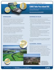
Figure 4: Image of 3 REMUS AUV CTD cast sites in Solomons, MD. Data were used to test Velocwincodethe cast was approximately 30 feet. Multiple copies of this downward cast were duplicated within the textle to create a test AUV CTD data le for which we could start writing code to pick the beginning andend of each sound speed prole cast. Here we assumed that each time the AUV began its decent it wouldrst come up to the surface (where it would have at some point a depth reading of zero), get a positionx, decend vertically down the water column to the seaoor, then travel to the next cast location andcome up again to the surface to repeat the process again. Once the Velocwin algorithm was manipulatedto account for these changes to split out the SSPs, we collected more data in May to test its durability.2.2 ExperimentFor the May 28 experiment in Solomons, MD on the NOAA S/V BAY HYDROGRAPHER, our majortask (after moding the Velocwin program to be able to accept the CTD sensor data from the AUV) wasto test this code with a simple, yet more typical, cast-like situation. We deployed the REMUS 100 toacquire three simultaneous sound speed casts within close proximity to one another (between 9-29 meters)on the BAY HYDROGRAPHER in Solomons (Figure 4). The CTD data output from the REMUS wasagain inserted in Velocwin. However, we noticed that our original assumption in which the depth readingwould be zero just before the downcast was incorrect. We had unfortunately used this assumption todetermine how to split up the text le of back-to-back CTD casts. Figure 5 illustrates also that as theAUV goes from one cast location to another, it oscillates along the seaoor. Our solution was to adjustthe Velocwin algorithm to incorporate box car averaging.Although this worked for the present dataset we were not certain whether it would work for others.7

Figure 5: Plot of CTD data acquired May 28 to test simplied code in Velocwin for extracting back-tobackcastsFurthermore, we wanted to increase the number of casts and the variability of locations so that oursampling would also take in to consideration both areas which were stratied and well mixed. Therefore,a second, larger dataset was acquired on July 8-9 to test the program's reliability and robustness and thisalso provided an opportunity to untilize the information gained from the Lagrangian particle trackingexercise as explained in section 2.1.1. We were particularly interested in looking at what the particleswere doing during the ooding and ebbing periods of the tidal cycles. We found that the tidal predictionsfrom CO-OPS suggest that the high tide occurred around 1200 GMT and the low tide around 1800 GMTon each day (Figure 6).The reason for looking at water elevations was because we felt that the tidal forces signicantly inuenced(along with the discharge from the river) the oceanographic dynamics (i.e. changes in temperatureand salinity distribution) in this particular area. Therefore we kept this in mind when looking at theoutcome of the particle simulation.Figure 7 shows two images: the one on the left is the horizontal movements of the tracked particlesand the one on the right shows their vertical motion, both of which are in the Solomons region. Theinitial locations of the particles are shown as rectangular boxes and each particle ensemble is imparteda dierent color for visual clarity. These plots clearly show the particle movements in time in both thehorizontal and vertical directions and the blue and magenta particles especially show a wide range ofmovements in the horizontal. This implies that an AUV initially positioned at the blue or magenta boxwould be aected signicantly by the tidal motion of the water column. The blue and the red particlesshow signicant vertical movements implying that an AUV acquiring CTD data at these locations wouldexperience vertical bueting forces. Therefore, we felt that during times of ooding and ebbing, therewould be well mixed as well as stratied areas to sample (in the shallow and deep areas) before and afterthe spit.8

Figure 6: Tides for Solomons, MD July 8-9, 2008Figure 7: July 8 at 10 am (EDT) where the left image is a top horizontal view of the particle movementand the right image is the verticle movement of the particles. In the left image each colored box representsthe point at which we 'dropped' particles into the ocean on June 26 (ie. their initial locations where theparticles began). The other colored regions are the particle locations on 10am on July 8. The blue boxis the region where we decided to collect CTD data.Cast locations (Figure 8) were also spread further apart than the May 28th set and at dierent depthsto try to mimick a mini-survey type area. This dataset consisted of six cast locations and the samplingtook place three times daily at each location at around high and then low tide. A total of 24 casts were9

taken each day.Figure 8: Priority 1 cast locations were acquired with the SBE FastCat 49 CTD on the REMUS AUVJuly 8 and priority 2 cast locations were acquired July 9. All casts were at three dierent times of thetidal cycleThe SBE 49 FastCAT CTD data was run through Velocwin to calculate the sound speed see if theindividual sound speed proles could be detected and split up from the others.3 Results3.1 Algorithm Results and RenementAfter assessing the data acquired from our July 8-9 experiment we found that 13 of the 24 casts takenon July 8 and 20 of the 24 casts taken July 9 were properly determined using a basic algorithm whichwas incorporated into Velocwin (Figure 9).10

Figure 9: This image is of the vertical track of the REMUS on July 8 (day number 190). In this imagesound speed casts acquired by the REMUS are indicated by the green circles. The downward dives thatwill be used to create a SSPs were detect using a basic algorithm. Note the beginning of the downwardcasts are in green squares and their respective ending locations are in magenta square (note: not manycasts are detected). Black curve indicates nominal bathymetry prole. The same is also true for Figure10. Please note for the remainer of this paper, each dive that travels all the way to the seaoor and isdetected by the algorithm will often be referred to as a sound speed cast since it is generally the samepattern as manually lowering a CTD.On closer inspection we noted that there were more casts acquired by the REMUS than we had inputinto the REMUS program. This was due to the emergency climbs which occur when the REMUS's sensordetects the seaoor unexpectedly rising beyond the set buer. In order to detect more sound speed casts,we rened the basic algorithm to take into consideration the local bathymetry.The basic downward cast detection algorithm works (for each cast) as follows:1. Remove any duplicate time/depth values and get a unique set of times and depths to work with,2. Find the global minimum (Hmin) and maximum (Hmax) depths of descent by the AUV and letD= Hmax - Hmin3. Specify a percentage, r (1%-5%) and examine to see when the AUV depths (as a function of time),h(t) satisfy the dual-inequality Hmin + rˆD ≤ h(t) ≤ Hmax + rˆD and if so, also whether sets ofthree consecutive depth values (h(t) itself, the values before and after it) generate average negativevertical descent speeds (ie. the AUV is sinking)4. Continue the iteration in 3 until either h is outside the depth range or the vertical descent speedreverts back to a positive value via zero (the latter condition is what usually occurs) and,11

5. Test to see whether the total depth descended by the AUV is greater than ½ˆ(Hmin+Hmax) ie.in excess of the midway point of the global AUV maximum descent depth.If condition 5 is true, then it is assumed that we have detected a valid downward cast.In the more advanced/rened algorithm, step 2 is replaced by calculating a time-varying bottom depth,H(t) following the horizontal trajectory of the AUV. This is achieved by using a bottom bathymetricsounding data set together with its (lon,lat) positions (from say the NGDC gridded bathymetric databaseor NOS scattered sounding data) and interpolating the bottom depth values to the (lon,lat) position ofthe AUV as a function of time. The interpolation is carried out using an inverse-square method as inthe creation of the bottom bathymetry for the ROMS model grid (section 2.1.1). Thereafter, step 3 ismodied where now the equivalent dual-inequality becomes r ˆH(t) ≤ h(t) ≤ (1-r)ˆH(t) and in step 5,the average bottom depth checked against is the mean of the two bottom depths when criteria 3 and 4are rst satised by h(t) and when they are last satised (before moving on to criterion 5). Therefore,this advanced algorithm checks the vertical position of the AUV relative to a more realistic bottombathymetry as opposed to a globally xed (maximal) descent depth as in the basic algorithm and itrequires as an input a bottom bathymetric data set containing (lon, lat, depth) vectors.A weakness in both algorithms is that in phase 3, if the AUV temporarily ascends up the water columneven momentarily, thus generating an averaged positive vertical velocity (or zero), it assumes that theAUV is no longer in descent and begins to test for criterion 5.Figure10 shows that this advanced algorithm unlike its basic counterpart (Figure 9) is able to detect allof the downward proles with any emergency climbs. As for climbs which begin in the middle of the watercolumn and proceed downward, they will not be considered for the sound speed uncertaintly calculationbut will be added to the temperature and salinity data les submitted to the National OceanographicData Center (NODC) of NOAA.12

Figure 10: This image is of the vertical track of the REMUS on July 8 (day number 190). This time thedownward casts acquired by the REMUS were detected by a rened algorithm using local bathymetry(black curve) and are indicated by the green circles. The purple circle indicates where the alorithm notesthe end of the cast. Note that all the sound speed proles programmed in the REMUS and additionalproles from emergency climbs were detected.3.2 Validating ROMSAfter running simulations from April 15, 2008 to July 15, 2008, temperature and salinty comparisonswere made between the data acquired by the REMUS and that of the simulation. For the CTD dataacquired July 8 we chose four AUV downward casts (cast numbers 6-9) to analyze and nine casts (castnumbers 11-19) acquired on July 9. Of those total 13 downward casts that we analyzed we chose three(illustrated by green dots in Figure 11) to explain for this paper.13

Figure 11: REMUS AUV track on left was done July 8, 2008 and track on right was done July 9, 2008.R1-R6 and B1-B6 were the original cast locations inserted into the REMUS AUV software so that theAUV would dive down at those locations. Cast #8, 13 and 16 (noted by the green dots) represent thelocations which were analysed where the AUV dove to the bottom and were analyzed. These locationswere not inserted in the REMUS software but this where the AUV experienced emergency climbs whenit felt it was getting too close to the seaoor.The vertical tracks of the three casts are also illustrated by check marks in Figure 12.14

Figure 12: Vertical path of REMUS on July 8 or day number 190 (left) and vertical path of REMUS onJuly 9 or day number 191 (right) . The three check marks on the left and right illustrate the three castswhose temperature and salinty proles will be shown below. Cast 8, 13 and 19 were purposely selectedto show if there are any dierences between the data acquired and that from the simulation for shallowand deep casts. The reason for the greater number of dives/casts in the data taken July 9 is because onJuly 8 new les were created for data acquired over each of the three tidal cycles to whereas the dataacquired on July 9 were all added to the same le.Looking at the salinity and temperature proles for casts 8 (Figure 13), 13 (Figure 14) and 16 (Figure14) we observed that AUV temperatures and salinities demonstrated the expected behavior of beingwarmer at ocean surface and saltier at ocean bottom as well being stratied. The data appears to bereliable and free of appreciable systemic measurement errors.15

Figure 13: Temperature and salinty proles acquired with the CTD on the REMUS (blue) and thosefrom ROMS predictions (red) for cast #8ROMS predictions reect the temperature and salinity observations from the REMUS and as expectedof numerical ocean models; it tends to underpredict the level of stratication in both temperature andsalinity especially at the surface and the bottom extremeties. The deviations of the ROMS predictionsFigure 14: Temperature and salinty proles acquired with the CTD on the REMUS (blue) and thosefrom ROMS predictions (red) for cast #13 (two left most graphs) and cast 16 (two right most graphs)from the AUV observations shown in Figures 13 and 14 are typical of all of the stations; temperaturedeviation is typically 0.5 degree celsius and salinity deviation is typically around one unit. These constant16

osets could be due to an initial oset in the initial conditions employed; from the WOA 2001 climatologyand/or the employment of the ROMS bulk ux formulation/approximation together with meteorologicalforcing from a forecast model (NAM12) as opposed to using observed data of a high a spatio-temporalnature. Sometimes the ROMS model depths and the those from the REMUS are shown to have somedierences and this is expected as the model depths were formed by numerical interpolation of multi-yearsounding data on a nite resolution horizontal grid.4 ConclusionIn this paper we demonstrated proof-of-concept use of an AUV and ROMS to acquire sound speed proles.This demonstration and experimention has allowed us to not only enhance our understanding of oceandynamics as hydrographers but it has also allowed us the ability to conduct a temperature and salinityvalidation excercise as well as learn how to 'smartly' use an AUV to acquire SSPs to avoid unecessarywear and tear on the instrument and sensor. Now we have the option to use an additional method (asidefrom using an MVP, digibar or manually lowering a CTD to acquired SSPs) to determine the projectareas' sound speed uncertainty (Imahori and Hiebert, 2008).For the purposes of our temperature and salinty validation exercise we found that the data from theREMUS was of good quality and free of systemic errors and that the data was useful for validating anocean model (ROMS) run under realistic conditions during the timeframe of July 8-9, 2008. We alsofound that ROMS appears to reect the REMUS data with constant osets in temperature and salinitybut these are not drastic.NOAA's future plans are to test and evaluate AUV SSP extraction algorithm again in Novemberof this year. This upcoming test will ensure that the original algorithm which was written in Fouriertransform was correctly translated to VB6 for the Velocwin program and will be ready for operational usenext eld season. Our work has been oriented toward characterizing the sound speed in a hydrographicproject area a priori. The potential exists to also "correct" for refraction eects seen in multibeam datapost a posteriori.It is important to note that the AUV used in this experiment is intended to be used for side scansonar surveys and was used as proof-of-concept. The AUV is larger, more complex, and more expensivethan necessary or practical for an AUV designed to collect only CTD data. NOAA anticipates that small,inexpensive AUV's would be used for operational deployment. Another point which future users shouldconsider is where best to use an AUV. To date we have been using the AUV where the vessel tracdoes not prevent the AUV from surfacing. In high trac areas, users have discussed the possibility ofnot allowing the AUV to surface but stay a few meters below the surface. If this is going to become astandard operating procedure, users should consider the reason why they need sound speed and how thesound speed varies much more within the rst 10 meters than typically in the rest of the prole. NOAAhas much work to do in this arena both on the operational and policy side. NOAA welcomes discussionswith other hydrographers using or looking to use AUVs in this manner.We hope the proof-of-concept testing will encourage more collaboration between NOAA hydrographyand marine modeling to further utilize all relevant information important to the problem domain. NOAAis looking into whether CSDL's Princeton Ocean Model System (POMS) for Cook Inlet and KachemakBay, AK can be used to help identify the oceanographic variability of the area. While there is no wayto say quantiably that the models are showing exactly where to sample, they give us more informationthan we currenlty have to understand the survey area as a whole. Hydrographers are not oceanographersbut can benet from their knowledge and tools. It is our hope that this use of models will make it possiblefor NOAA to some day design survey sheet limit (sub) areas based on tidal and sound speed bound areas17

ather than arbitrary rectangle boxes (which are currently being used), thereby reducing some of thetidal and sound speed issues that hydrographers have to deal with occassionally.4.1 AcknowledgmentsMary Erickson, LCDR EJ Vandenameele, Kathryn Ries, Je Ferguson, Crescent Moegling, Jack Riley,Michael Davidson, Vitad Pradith, Corey Allen, and Mike Annis.ReferencesBecker, R. and Grim, P. (1989). Sound velocity products for NOS hydrography. In Proceedings from theCanadian Hydrographic Conference,Vancouver, BC, Canada.Berliand, M. and Berliand, T. G. (1952). Determining the net longwave radiation of the earth withconsideration of the eects of cloudiness (in russian). Izv. Akad. Nauk SSSR, Ser. Geoz 1.Conkright, M. E., P.Locarnini, R., Garcia, H. E., Brian, T. D. O., Boyer, T. P., Stephens, C., andAnotonov, J. I. (2002). World ocean atlas 2001 : Objective analyses, data statistics, and gures.CD-ROM Documentation. National Oceanographic Data Center, Silver Spring, MD, pp. 17.Delft3D (2008). grid generator. http://delftsoftware.wldelft.nl/.Imahori, G. (2007). Case studies of space and time variability in sound speed: An investigation intothe sound speed component of total depth uncertainty using NOAA Ship Fairweather data. Technicalreport, Unversity of New Hampshire, Center for Coast and Ocean Mapping - Joint HydrographicCenter.Imahori, G. and Hiebert, J. (2008). An algorithm for estimating the sound speed component of todepth uncertainty. In Proceedings of the Canadian Hydrographic Conference and National SurveyorsConference.Liu, W. T., Katsaros, K. B., and Businger, J. (1979). Bulk parameterization of the air-sea exchangeof heat and water vapor including the molecular constraints at the interface. Journal of AtmosphericSciences, 36:17221735.Luettich, R., Westerink, J. J., and Schener, N. W. (1992). Adcirc: an advanced three-dimensionalcirculation model for shelves coasts and estuaries, report 1: theory and methodology of adcirc-2ddiand adcirc-3dl. Technical report, Dredging Research Program Technical Report DRP-92-6, U.S. ArmyEngineers Waterways Experiment Station, Vicksburg, MS, 137p.Mellor, G. L. and Yamada, T. (1982). Development of a turbulence closure model for geophysical uidproblems. Reviews of Geophysics and Space Physics, 20:851875.Shchepetkin, A. F. and McWilliams, J. C. (1998). Quasi-monotone advection schemes based on explicitlocally adaptive dissipation. Monthly Weather Review, 126:15411580.Shchepetkin, A. F. and McWilliams, J. C. (2003). A method for computing horizontal pressure-gradientforcing in an oceanic model with a nonaligned vertical coordinate. Journal of Geophysical Research,108:134.18

Shchepetkin, A. F. and McWilliams, J. C. (2004). The regional oceanic modeling system : a split-explicit,free-surface, topography-following-coordinate ocean model. Ocean Modeling, 9:347404.Song, Y. T. and Haidvogel, D. B. (1994). A semi-implicit ocean circulation model using a generalizedtopography following coordinate system. Journal of Computational Physics, 115:228244.Styles, R. and Glenn, S. M. (2000). Modeling stratied wave and current bottom boundary layers in thecontinental shelf. Journal of Geophysical Research, 105:2411924139.Warner, J. C., Sherwood, C. R., Arango, H. G., and P.Signell, R. (2005). Performance of four turbulenceclosure methods implemented using a generic length scale method. Ocean Modeling, 8:81113.19