Wind in complex terrain. A comparison of WAsP and two ... - WindSim
Wind in complex terrain. A comparison of WAsP and two ... - WindSim
Wind in complex terrain. A comparison of WAsP and two ... - WindSim
- No tags were found...

You also want an ePaper? Increase the reach of your titles
YUMPU automatically turns print PDFs into web optimized ePapers that Google loves.
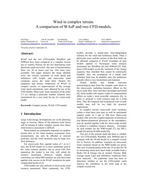
<strong>W<strong>in</strong>d</strong> <strong>in</strong> <strong>complex</strong> terra<strong>in</strong>.A <strong>comparison</strong> <strong>of</strong> <strong>WAsP</strong> <strong>and</strong> <strong>two</strong> CFD-models.Erik Berge Arne R. Gravdahl Jan Schell<strong>in</strong>g Lars Tallhaug Ove UndheimKjeller V<strong>in</strong>dteknikk AS Vector AS Hydro Oil & Energy Kjeller V<strong>in</strong>dteknikk AS Institutt for energiteknikk*erik.berge@v<strong>in</strong>dteknikk.no gravdahl@vector.no jan.schell<strong>in</strong>g@hydro.com lars.tallhaug@v<strong>in</strong>dteknikk.no ove.undheim@v<strong>in</strong>dteknikk.no*Presently at Kjeller V<strong>in</strong>dteknikk ASAbstract:<strong>WAsP</strong> <strong>and</strong> the <strong>two</strong> CFD-models <strong>W<strong>in</strong>d</strong>Sim <strong>and</strong>3D<strong>W<strong>in</strong>d</strong> have been compared at a <strong>complex</strong> terra<strong>in</strong>site <strong>in</strong> western Norway for the <strong>two</strong> dom<strong>in</strong>at<strong>in</strong>g w<strong>in</strong>ddirections south <strong>and</strong> north. One year <strong>of</strong> measurementsfrom <strong>two</strong> 50 m masts <strong>and</strong> one 10m mast wereavailable. The paper analyses the mean absoluteerror, the vertical variations <strong>of</strong> w<strong>in</strong>d speed <strong>and</strong>turbulence with height, <strong>and</strong> meso-scale w<strong>in</strong>dvariations across the w<strong>in</strong>d farm. Despite thesimplicity <strong>and</strong> known weaknesses <strong>of</strong> <strong>WAsP</strong> <strong>in</strong><strong>complex</strong> terra<strong>in</strong>, no improvements <strong>of</strong> the averagew<strong>in</strong>d speed calculations were obta<strong>in</strong>ed by use <strong>of</strong> theCFD-models. Meso-scale w<strong>in</strong>d variations <strong>of</strong> the order2-3 m/s dur<strong>in</strong>g a particular weather situation wereencountered for a case study by use <strong>of</strong> a meso-scalemodel.Keywords: Complex terra<strong>in</strong>, <strong>WAsP</strong>, CFD-models.1 IntroductionLarge w<strong>in</strong>d energy developments are at the plann<strong>in</strong>gstage <strong>in</strong> Norway. Many <strong>of</strong> the planned w<strong>in</strong>d farmswill be located <strong>in</strong> rather <strong>complex</strong> coastal sites wherew<strong>in</strong>d resource assessment is difficult.<strong>W<strong>in</strong>d</strong> models are potentially important at <strong>complex</strong>terra<strong>in</strong> sites <strong>in</strong> the w<strong>in</strong>d resource assessment s<strong>in</strong>cemeasurements can only be afforded at selectedpositions, <strong>and</strong> the w<strong>in</strong>d variations may be large overshort distances.For micro-scale flow (spatial scales <strong>of</strong> 1 m to 2km), the <strong>WAsP</strong> model [1] is most commonly used <strong>in</strong>the w<strong>in</strong>d resource analysis, but <strong>in</strong> areas with flowseparation the model is not very well suited forresource assessment. However, simple terra<strong>in</strong>corrections (so called RIX-analysis see [2]) have beenapplied with success to the <strong>WAsP</strong> simulation for quitecomplicated terra<strong>in</strong> [2,3].CFD-models are also utilized <strong>in</strong> micro-scale w<strong>in</strong>dresource assessment. Most commonly, the CFDmodelsdevelop a steady-state time-<strong>in</strong>dependentsolution for the w<strong>in</strong>d <strong>and</strong> turbulence fields. Thus, aphysically more realistic picture <strong>of</strong> the flow field canbe obta<strong>in</strong>ed compared to <strong>WAsP</strong>. Examples <strong>of</strong> suchmodels applied to Norwegian w<strong>in</strong>d resourceassessment are <strong>W<strong>in</strong>d</strong>Sim [4] <strong>and</strong> 3D<strong>W<strong>in</strong>d</strong> [5]. Still,these CFD-models avoid the <strong>in</strong>clusion <strong>of</strong> the energyequation, thus stratified flow cannot be realisticallyh<strong>and</strong>led. Also, the assumption <strong>of</strong> a steady stateturbulent field may be doubtful s<strong>in</strong>ce the turbulenceactually <strong>of</strong>ten is very <strong>in</strong>termittent <strong>and</strong> transient.Nested models that h<strong>and</strong>le real-timemeteorological data from the synoptic scale down tothe micro-scale, <strong>in</strong>clud<strong>in</strong>g buoyancy effects on themicro-scale flow, have also been developed <strong>and</strong> tested[6]. Such models still require weeks <strong>of</strong> computationalefforts on today’s most powerful computers [6], <strong>in</strong>order to generate a w<strong>in</strong>d resource map for a w<strong>in</strong>dfarm. Thus the temporal <strong>and</strong> economical costs <strong>of</strong> suchmodels may still be too high for practicalapplications.In <strong>complex</strong> terra<strong>in</strong>, meso-scale w<strong>in</strong>d variationswith<strong>in</strong> a w<strong>in</strong>d farm area may as well be anticipated(spatial scales <strong>of</strong> 2 km to 200 km). Meso-scalemodels, that solve the coupled equations <strong>of</strong> dynamical<strong>and</strong> thermo-dynamical processes <strong>in</strong> the atmosphere,may be needed together with the micro-scale modelsto achieve a complete resource analysis. Exampleson such models are the WRF-model [7], the MC2-model [8] <strong>and</strong> the RAMS-model [9].The aim <strong>of</strong> the present study has been to validatethe <strong>two</strong> CFD-models <strong>W<strong>in</strong>d</strong>Sim <strong>and</strong> 3D<strong>W<strong>in</strong>d</strong> <strong>and</strong> tocompare with the <strong>WAsP</strong> model at a <strong>complex</strong> terra<strong>in</strong>site <strong>in</strong> Norway. In addition, examples on meso-scalew<strong>in</strong>d variations based on the WRF-model are given.One year <strong>of</strong> measurements from one 10 m <strong>and</strong> <strong>two</strong> 50m measur<strong>in</strong>g masts have been made available from aHydro Oil & Energy site <strong>in</strong> western Norway. Bothaverage mean w<strong>in</strong>d <strong>and</strong> turbulence conditions havebeen analyzed. An important issue has been todeterm<strong>in</strong>e whether or not the CFD-models couldimprove the confidence <strong>in</strong> the w<strong>in</strong>d map at the<strong>complex</strong> terra<strong>in</strong> site.
2 Measur<strong>in</strong>g program2.1 The Gurskøy regionHydro Oil & Energy <strong>in</strong>itiated <strong>in</strong> 2000 a fieldmeasur<strong>in</strong>g campaign at Gurskøy <strong>in</strong> western Norway.The area is located about 25 km east <strong>of</strong> Stadt, one <strong>of</strong>the w<strong>in</strong>diest regions <strong>in</strong> Norway. The Gurskøy isl<strong>and</strong>has a complicated local terra<strong>in</strong> structure withmounta<strong>in</strong>tops <strong>of</strong> about 600 m with steep edges downto local valleys <strong>and</strong> fjords (see Figure 1).Considerable local flow separation is expected <strong>in</strong> thistype <strong>of</strong> terra<strong>in</strong>. From the sectors W to N open oceanflow modified by the local terra<strong>in</strong> may be expected.Toward S <strong>and</strong> E high mounta<strong>in</strong>s <strong>of</strong> 800-1500 m areencountered at distances <strong>of</strong> approximately 15 km ormore, with associated meso-scale w<strong>in</strong>d effects.2.2 Description <strong>of</strong> the measur<strong>in</strong>g sitesThe measurements were collected from april 2002 tomay 2003 for the sites 1 (z=424 m), 2 (z=390 m) <strong>and</strong>3 (z=352 m) (see Figure 1). At site 1, themeasurements were carried out with a 10 m steel tubemast, while 50 m steel tube masts where employed atsites 2 <strong>and</strong> 3.The w<strong>in</strong>d speed measurements were collected withthe NRG Maximum #40 anemometer. Comparisonwith RISØ w<strong>in</strong>d speed sensors have shown that theNRG sensor underestimates the w<strong>in</strong>d speed for w<strong>in</strong>dspeeds lower than 2 m/s. For an annual average w<strong>in</strong>dspeed <strong>in</strong> the range 7-9 m/s the underestimation willbe about 0.04 m/s, i.e. much less than the overalluncerta<strong>in</strong>ty <strong>of</strong> the measurements, <strong>in</strong>clud<strong>in</strong>g theuncerta<strong>in</strong>ties <strong>of</strong> long-term variability <strong>of</strong> the w<strong>in</strong>d, <strong>of</strong>about 5% (see [3]).The w<strong>in</strong>d rose at site 1 is presented <strong>in</strong> Figure 2.We note the dom<strong>in</strong>ance <strong>of</strong> w<strong>in</strong>ds from S <strong>and</strong> SW <strong>and</strong>N <strong>and</strong> NE.The sites 1 <strong>and</strong> 2 are situated on an east-westridge with considerable speed-up for both southerly<strong>and</strong> northerly flow. The hillside to the south stretchesall the way down to the fjord, while a mounta<strong>in</strong> risesto about 400 m further to the south. Turbulence couldbe expected at all three sites north <strong>of</strong> this mounta<strong>in</strong>for the dom<strong>in</strong>at<strong>in</strong>g southerly flow. At site 1 there issome shelter<strong>in</strong>g toward W <strong>and</strong> NW, but this is a w<strong>in</strong>d
Figure 1: Location <strong>of</strong> the three measur<strong>in</strong>g sites 1, 2 <strong>and</strong> 3 at the Gurskøy isl<strong>and</strong>. Height contours are for every 20m.direction with low frequency. Site 2 is partly shelteredfor the direction NE. Site 3 is located <strong>in</strong> a SW to NEoriented hillside. Speed-up for SW flow can beexpected at this site. The w<strong>in</strong>d rose is consistent withobservations from other stations <strong>in</strong> this region.270300240Expected Long−Term <strong>W<strong>in</strong>d</strong> Rose at 3043302100180Figure 2: <strong>W<strong>in</strong>d</strong> rose at site 1.30600.05 0.1 0.15 0.2 0.253 Micro-scale model set-up3.1 <strong>WAsP</strong>1501209025 −>20 − 2515 − 2010 − 155 − 100 − 5<strong>WAsP</strong> version 8.1 was employed <strong>in</strong> this study. Heightcontours for each 5 m were available for an area <strong>of</strong>about 3km*3km cover<strong>in</strong>g the met mast. Outside thisarea 20 m height contours were used. A backgroundroughness <strong>of</strong> 0.03 m describ<strong>in</strong>g the bare mounta<strong>in</strong>areas, was applied. Higher roughness values wereapplied to forests <strong>and</strong> small towns.3.2 The CFD-models<strong>W<strong>in</strong>d</strong>Sim 3D<strong>W<strong>in</strong>d</strong>Size <strong>of</strong> model doma<strong>in</strong> 20*20 17*14(km 2 )Total number <strong>of</strong> cells 144*111*20 142*160*48Size <strong>of</strong> model doma<strong>in</strong> 3*2 1.44*2.22with 30m resolution(km 2 )Number <strong>of</strong> cells with 100*67 48*7430m resolutionHeight (m) <strong>of</strong> the lowestlayers6, 20, 36, 57 7, 15, 24,33, 44Number <strong>of</strong> layers <strong>in</strong> the 20 48verticalHeight (m) <strong>of</strong> the model 2500 5000Boundary conditions (seetext for explanation)Coriolis force No YesTurbulent scheme k-ε k-εTable 1: Set-up <strong>of</strong> <strong>W<strong>in</strong>d</strong>Sim <strong>and</strong> 3Dw<strong>in</strong>d for thesimulation.The details <strong>of</strong> the model set-up for the <strong>two</strong> CFDmodelsare compared <strong>in</strong> Table 1.Although an as similar set-up as possible has beenthe <strong>in</strong>tention, <strong>in</strong>evitably some differences are found.Both <strong>W<strong>in</strong>d</strong>Sim (for a documentation <strong>of</strong> <strong>W<strong>in</strong>d</strong>Simsee http://w<strong>in</strong>dsim.com) <strong>and</strong> 3D<strong>W<strong>in</strong>d</strong> [5], [10] arew<strong>in</strong>d flow solvers based on the 3D ReynoldsAveraged Navier-Stokes equations. The models solvethe atmospheric flow for a “steady-state” case for achosen w<strong>in</strong>d direction. By “steady-state” it is meantthat the model is run until the solution converges toone w<strong>in</strong>d <strong>and</strong> turbulence distribution for the entiredoma<strong>in</strong> that do not vary outside a pre-set convergencelimit. By simulat<strong>in</strong>g for several different w<strong>in</strong>ddirections (sectors) an annual average w<strong>in</strong>d speed canbe generated. The models are run for a given set <strong>of</strong>constructed boundary <strong>and</strong> <strong>in</strong>itial conditions. The k-εturbulence closure scheme is applied <strong>in</strong> both models.An important advantage <strong>of</strong> a CFD-modelcompared to <strong>WAsP</strong> is that the CFD-model calculatesthe turbulent quantities <strong>of</strong> the flow, <strong>and</strong> thus gives<strong>in</strong>formation about high turbulence areas that shouldbe omitted for w<strong>in</strong>d power exploitation. Also, thedirect effects <strong>of</strong> turbulence on the mean flow arecalculated. Especially <strong>in</strong> <strong>complex</strong> terra<strong>in</strong>, where acomplicated turbulence structure is encountered,benefits <strong>of</strong> a CFD-model are expected. However, anyturbulence model<strong>in</strong>g will <strong>in</strong>evitable <strong>in</strong>troduce newparameterization assumptions <strong>and</strong> constants, whichalso <strong>in</strong>troduces uncerta<strong>in</strong>ty <strong>in</strong> the model<strong>in</strong>g (see forexample [11]). Considerable uncerta<strong>in</strong>ty is thereforel<strong>in</strong>ked to the quantification <strong>of</strong> the turbulence <strong>and</strong> itseffects on the mean flow.Most CFD-models assume a neutral stratification<strong>of</strong> the atmosphere. For strong w<strong>in</strong>ds this is <strong>of</strong>ten agood approximation. But even for w<strong>in</strong>d speeds up to10-15 m/s stable stratification has been observed, atleast <strong>in</strong> the coastal areas <strong>in</strong> central Norway [12].Vertical w<strong>in</strong>d shears, turbulent fields etc. maydevelop quite differently dur<strong>in</strong>g stable (or unstable)conditions [12]. Thus, a limitation <strong>in</strong> the CFDapproachis encountered here. Another limit<strong>in</strong>g factoris the f<strong>in</strong>ite number <strong>of</strong> directions applied <strong>in</strong> thederivation <strong>of</strong> the annual average w<strong>in</strong>d speed. S<strong>in</strong>cethe long-term w<strong>in</strong>d speed is composed <strong>of</strong> w<strong>in</strong>d flowsfrom all different directions (though with somepredom<strong>in</strong>ant directions), a sample <strong>of</strong> for example 12sectors may be too small to represent an annualaverage properly.
4 ResultsThe CFD-models are <strong>in</strong>itialized based on assumptionsabout higher level (~500m) <strong>and</strong> lateral boundary levelw<strong>in</strong>d speed <strong>and</strong> pr<strong>of</strong>iles. A logarithmic w<strong>in</strong>d pr<strong>of</strong>ile(correspond<strong>in</strong>g to neutral stability conditions) isemployed at the boundaries <strong>in</strong> both models. Thus, <strong>in</strong>order to compare the output <strong>of</strong> the CFD-models withany measurements, the modeled w<strong>in</strong>d speed fieldshave to be scaled by use <strong>of</strong> the measurements. Forexample, for a specific annual w<strong>in</strong>d speed from sectorS at 50 m at one <strong>of</strong> the sites, the output <strong>of</strong> the CFDmodelwill be assumed equal to the measurement atthis site. It is then further assumed that the w<strong>in</strong>d fieldcan be scaled l<strong>in</strong>early based on the scal<strong>in</strong>g at thisparticular site. By employ<strong>in</strong>g this method modelsimulations <strong>of</strong> the w<strong>in</strong>d speed at all the measur<strong>in</strong>gsites can be obta<strong>in</strong>ed. Thus it is assumed that the ratio<strong>of</strong> the modeled <strong>and</strong> measured values at one site willapply to the whole model<strong>in</strong>g doma<strong>in</strong>. Thisassumption may not be valid everywhere <strong>in</strong> themodel<strong>in</strong>g doma<strong>in</strong>, but it is quite commonly applied tomodel<strong>in</strong>g. In the follow<strong>in</strong>g section we assess themodel simulations by us<strong>in</strong>g this method. The CFDmodelsare scaled to yield correct w<strong>in</strong>d speed at the50 m level at Site 2 <strong>and</strong> Site 3 respectively, then theresults at the other measur<strong>in</strong>g sites are extracted fromthe CFD-models.The <strong>WAsP</strong> model work differently. In order tomake the results from <strong>WAsP</strong> comparable to the CFDmodels,the measurements at 50 m from Site 2 <strong>and</strong>Site 3 are <strong>in</strong>serted <strong>in</strong> the model <strong>and</strong> the w<strong>in</strong>d speed <strong>of</strong>the other measur<strong>in</strong>g mast are obta<strong>in</strong>ed for the samesectors as utilized by the CFD-models.Note that the CFD-models were run only for the<strong>two</strong> sectors north (N) <strong>and</strong> south (S) to savecomputational efforts. Each sector covers 30°centered around 360° <strong>and</strong> 180° respectively.Accord<strong>in</strong>g to the w<strong>in</strong>d rose (see Figure 2), thedirections N <strong>and</strong> S represent ca. 13% <strong>and</strong> 18% <strong>of</strong> thew<strong>in</strong>d data respectively.4.1 Annual average w<strong>in</strong>d speedIn Figure 3 the vertical pr<strong>of</strong>iles at site 2 have beenobta<strong>in</strong>ed based on a “true” solution at 50 m height atsite 3. For the southerly sector the w<strong>in</strong>d direction isnearly perpendicular to the steep slope to the south <strong>of</strong>site 2 <strong>and</strong> a strong speed-up is encountered. Both<strong>W<strong>in</strong>d</strong>Sim <strong>and</strong> <strong>WAsP</strong> yield only small differencesfrom the observations, while 3D<strong>W<strong>in</strong>d</strong> yields a largeoverestimation <strong>of</strong> the w<strong>in</strong>d speed. For the northerlysector, the w<strong>in</strong>d speed actually decreases from 10 mto 50 m at site 2. All three models underestimate thew<strong>in</strong>d speed for this sector, still <strong>WAsP</strong> yields the bestresults <strong>in</strong> this particular case.A further <strong>comparison</strong> <strong>of</strong> the output <strong>of</strong> the modelsimulations with the observations has been carried out. Thethree models are all scaled to fit the observations at 50 mheight at either site 2 or site 3.Based on the scaled values <strong>of</strong> each <strong>of</strong> the <strong>two</strong> sites,the annual average w<strong>in</strong>d speed is estimated at theother levels <strong>of</strong> the same mast (10m <strong>and</strong> 30m) <strong>and</strong>Height (m)Height (m)605040302010Site 2 - S (scaled at site 3 50m)00.00 0.50 1.00 1.50 2.00605040302010Scaled w<strong>in</strong>dspeedSite 2 - N (scaled at site 3 50m)00.00 0.50 1.00 1.50 2.00Scaled w<strong>in</strong>dspeedOBSWASPWINDSIM3D<strong>W<strong>in</strong>d</strong>OBSWASPWINDSIM3D<strong>W<strong>in</strong>d</strong>Figure 3. Scaled vertical pr<strong>of</strong>iles at Site 2 for sector S(upper panel) <strong>and</strong> sector N (lower panel).Modelled2.001.801.601.401.201.000.800.600.400.200.00Obs vs model Sector S0.00 0.20 0.40 0.60 0.80 1.00 1.20 1.40 1.60 1.80 2.00ObservedWasp WINDSIM 3D<strong>W<strong>in</strong>d</strong>
2.001.801.601.40Obs vs model Sector Nresults underl<strong>in</strong>e that a RIX-correction should alwaysbe supported by empirical data, <strong>and</strong> a generalization<strong>of</strong> the method from one area to another is notrecommended.Modelled1.201.000.800.600.400.200.000.00 0.20 0.40 0.60 0.80 1.00 1.20 1.40 1.60 1.80 2.00ObservedWasp WINDSIM 3D<strong>W<strong>in</strong>d</strong>Figure 4. Observed vs. modelled annual normalizedw<strong>in</strong>d speed for sector S (upper panel) <strong>and</strong> sector N(lower panel).at the three measur<strong>in</strong>g levels <strong>of</strong> the other 50m mast<strong>and</strong> f<strong>in</strong>ally at 10 m at site 1. The results aresummarized <strong>in</strong> Figure 4 <strong>and</strong> Table 2. The totalnumber <strong>of</strong> data po<strong>in</strong>ts<strong>WAsP</strong>S<strong>W<strong>in</strong>d</strong>-Sim S3D-<strong>W<strong>in</strong>d</strong> S<strong>WAsP</strong>N<strong>W<strong>in</strong>d</strong>-Sim N3D-<strong>W<strong>in</strong>d</strong>NMAE 0.11 0.10 0.28 0.14 0.24 0.24COR 0.88 0.84 0.74 0.89 0.58 0.79Table 2: Mean Absolute Error (MAE) <strong>and</strong> correlationcoefficient (COR) <strong>of</strong> ratios between models <strong>and</strong>measurement. Each statistical parameter is based on12 data values.to be verified are 12, thus any statistical analysis hasto be <strong>in</strong>terpreted with care s<strong>in</strong>ce the data po<strong>in</strong>ts arefew. For the sector S, <strong>WAsP</strong> <strong>and</strong> <strong>W<strong>in</strong>d</strong>Sim showsimilar behavior, while the errors are somewhatlarger for 3D<strong>W<strong>in</strong>d</strong>. For sector N, <strong>WAsP</strong> givessomewhat surpris<strong>in</strong>gly the best correspondence, while<strong>W<strong>in</strong>d</strong>Sim has the lowest correlation. Based on theresults <strong>of</strong> Figure 3 <strong>and</strong> 4 <strong>and</strong> Table 2 we concludethat the errors are as large (<strong>and</strong> actually a littlelarger) for the CFD-models compared to <strong>WAsP</strong> forthe <strong>two</strong> sectors analyzed. This is an importantf<strong>in</strong>d<strong>in</strong>g, although we lack <strong>in</strong>sight <strong>in</strong>to the reasonswhy the CDF-models are unable to improve thesimulations at Gurskøy. In the follow<strong>in</strong>g sections wepresent a discussion aim<strong>in</strong>g to give a betterunderst<strong>and</strong><strong>in</strong>g <strong>of</strong> the model<strong>in</strong>g results.A RIX-analysis was carried out for the three sitesto check if the <strong>WAsP</strong> results could be improved. TheRIX-values us<strong>in</strong>g a radius <strong>of</strong> 2 km were 24.2%, 20%<strong>and</strong> 17.2% for the site 1, site 2 <strong>and</strong> site 3 respectively.In contrast to [3] no relationship between thedifferences <strong>in</strong> RIX-values <strong>and</strong> the prediction errorwas found. For example, employ<strong>in</strong>g the 10 mmeasurements at site 1 gave an over prediction <strong>of</strong> thew<strong>in</strong>d speed at site 2 <strong>and</strong> 3, while an under predictioncould be expected from the RIX-analysis. These4.2 Turbulence <strong>and</strong> the directionaldependenceIn Figure 5 the turbulence <strong>in</strong>tensities at site 3 ispresented. While 3D<strong>W<strong>in</strong>d</strong> overestimates theturbulence for sector S <strong>W<strong>in</strong>d</strong>Sim gives too low values.For sector N both models are closer to theobservations, but still 3D<strong>W<strong>in</strong>d</strong> over predicts while<strong>W<strong>in</strong>d</strong>Sim under predicts. The same pattern isencountered for site 2 (not shown), <strong>and</strong> <strong>in</strong> othersimilar model experiments us<strong>in</strong>g 3D<strong>W<strong>in</strong>d</strong>. Ourconclusion from these <strong>in</strong>vestigations is that the overprediction <strong>of</strong> the turbulence <strong>in</strong> 3D<strong>W<strong>in</strong>d</strong> at site 3 mostprobable is l<strong>in</strong>ked to an underestimation <strong>of</strong> theaverage w<strong>in</strong>d speed at the same site. This also leadsto the overestimation <strong>of</strong> the predicted average w<strong>in</strong>dspeed level <strong>of</strong> 3D<strong>W<strong>in</strong>d</strong> at site 2 based on the w<strong>in</strong>dfield scale to site 3 (upper panel <strong>of</strong> Figure 3). InFigure 6 the turbulence pattern derived from 3D<strong>W<strong>in</strong>d</strong>is presented for the w<strong>in</strong>d directions 180° <strong>and</strong> 190°.Separated flow <strong>and</strong> strong turbulence is developed onthe lee side <strong>of</strong> the mounta<strong>in</strong> to the south <strong>of</strong> the ridgewhere the three meteorological masts are located. Atboth sites 2 <strong>and</strong> 3 it is likely that the turbulence<strong>in</strong>tensities could be rather sensitive to the exact w<strong>in</strong>ddirection.From Figure 7 it is also noted that the annualaverage w<strong>in</strong>d speed varies largely for different w<strong>in</strong>dspeed directions. The variability at site 2 for thedirection 170°, 180° <strong>and</strong> 190° is quite well capturedby 3D<strong>W<strong>in</strong>d</strong>. It is also observed that the outcome <strong>of</strong>Height (m)605040302010Site 3 sector S00 0.05 0.1 0.15 0.2 0.25 0.3Turbulence <strong>in</strong>tensityObs <strong>W<strong>in</strong>d</strong>SIM 3D<strong>W<strong>in</strong>d</strong>
Height(m)Site 3 sector N60504030201000 0.05 0.1 0.15 0.2 0.25 0.3Turbulence <strong>in</strong>tensity1.801.601.401.201.000.800.600.400.20Site 1Site 2Site 33D<strong>W<strong>in</strong>d</strong> at Site 2<strong>W<strong>in</strong>d</strong> speed dur<strong>in</strong>g the period April 2002 to May 2003Obs <strong>W<strong>in</strong>d</strong>SIM 3D<strong>W<strong>in</strong>d</strong>Figure 5: Observed vs. modeled turbulence <strong>in</strong>tensityat Site 3.the CFD-model is largely dependent on the selection<strong>of</strong> sectors. In the present case with <strong>complex</strong> terra<strong>in</strong> 12sectors yield <strong>in</strong>evitable to course resolution. Ideally atleast 36 sectors should be utilized, which on the otherh<strong>and</strong> <strong>in</strong>crease the computational dem<strong>and</strong>s.5. Comparison <strong>of</strong> the CFD modeldataIn Figure 8 the differences between <strong>W<strong>in</strong>d</strong>Sim <strong>and</strong>3D<strong>W<strong>in</strong>d</strong> for southerly flow are presented. The w<strong>in</strong>d6.9096.908x 10 6Turbulence Intensity []10.000 3 6 9 12 15 18 21 24 27 30 33 36DirectionFigure 7: <strong>W<strong>in</strong>d</strong> speed as a function direction scaledby the annual average w<strong>in</strong>d speed at 50 m at site 2.fields <strong>of</strong> the <strong>two</strong> models have been scaled <strong>in</strong> order tom<strong>in</strong>imize the differences between the <strong>two</strong> models.Note that dur<strong>in</strong>g the scal<strong>in</strong>g l<strong>in</strong>earity is assumed,although this may not strictly be the case. From thefigure we see quite much higher w<strong>in</strong>d speeds <strong>in</strong><strong>W<strong>in</strong>d</strong>Sim than <strong>in</strong> 3D<strong>W<strong>in</strong>d</strong> especially <strong>in</strong> the turbulentlee wakes. This is consistent with the f<strong>in</strong>d<strong>in</strong>gs <strong>in</strong>section 4.2 where a higher turbulent level isencountered <strong>in</strong> 3D<strong>W<strong>in</strong>d</strong>. This will reduce thehorizontal w<strong>in</strong>d speed, s<strong>in</strong>ce a larger part <strong>of</strong> theavailable k<strong>in</strong>etic energy <strong>of</strong> the flow is consumed byturbulent processes. Although the <strong>two</strong> models employthe same turbulent scheme we encounter a largedifference <strong>in</strong> the result<strong>in</strong>g w<strong>in</strong>d field <strong>and</strong> turbulence0.96.9070.8North<strong>in</strong>g [UTM EUREF89 sone 32]6.9066.9056.904HaugshornetLitlabøhornetHornelva0.70.60.50.46.9030.36.9020.26.9010.13.2 3.21 3.22 3.23 3.24 3.25 3.26 3.27 3.28 3.29East<strong>in</strong>g [UTM EUREF89 sone 32]x 10 5x 10 6Turbulence Intensity []6.90916.9080.96.9070.8North<strong>in</strong>g [UTM EUREF89 sone 32]6.9066.9056.9046.9036.9026.901HaugshornetLitlabøhornetHornelva3.2 3.21 3.22 3.23 3.24 3.25 3.26 3.27 3.28 3.29East<strong>in</strong>g [UTM EUREF89 sone 32]x 10 5Figure 6: Turbulence <strong>in</strong>tensities for w<strong>in</strong>d from 180°(upper panel) <strong>and</strong> 190° (lower panel) based on3D<strong>W<strong>in</strong>d</strong> model runs.0.70.60.50.40.30.20.1Figure 8: <strong>W<strong>in</strong>d</strong>Sim – 3D<strong>W<strong>in</strong>d</strong> at 50 m for sector S.field. This emphasizes the importance <strong>of</strong> the turbulentprocesses <strong>in</strong> rough terra<strong>in</strong> <strong>and</strong> the <strong>complex</strong>ity <strong>of</strong> aproper model<strong>in</strong>g <strong>of</strong> the turbulence.The frequency distribution <strong>of</strong> the w<strong>in</strong>d speedscover<strong>in</strong>g the doma<strong>in</strong> <strong>of</strong> Figure 8 is presented <strong>in</strong>Figure 9. The w<strong>in</strong>d speed <strong>of</strong> each s<strong>in</strong>gle grid-po<strong>in</strong>t at50 m <strong>in</strong> the model<strong>in</strong>g doma<strong>in</strong> has been <strong>in</strong>cluded <strong>in</strong>this distribution. The data are not scaled <strong>and</strong> therebynot strictly comparable, still a good picture <strong>of</strong> thebehavior <strong>of</strong> the <strong>two</strong> models is given. We immediatelyobserve the much higher frequency <strong>of</strong> low w<strong>in</strong>d
Figure 10: Outer doma<strong>in</strong> (red) <strong>and</strong> <strong>in</strong>ner doma<strong>in</strong>(blue) <strong>of</strong> the meso-scale simulation.The present analysis shows that, despite the<strong>complex</strong> terra<strong>in</strong>, <strong>WAsP</strong> compares better than theCFD-models to the observations when results for thesectors south <strong>and</strong> north are considered. Thisconclusion is valid both for the vertical w<strong>in</strong>d pr<strong>of</strong>iles<strong>and</strong> the annual average w<strong>in</strong>d speed levels. The meanabsolute error for sector south is 11%, 10% <strong>and</strong> 28%for <strong>WAsP</strong>, <strong>W<strong>in</strong>d</strong>Sim <strong>and</strong> 3D<strong>W<strong>in</strong>d</strong> respectively. Forsector north the correspond<strong>in</strong>g numbers are 14%,24% <strong>and</strong> 24%. The RMS-differences <strong>in</strong> the w<strong>in</strong>dspeeds between the <strong>two</strong> CFD-models have beencalculated for an area where w<strong>in</strong>d energy exploitationis realistic. For both sector south <strong>and</strong> north anaverage RMS-difference <strong>of</strong> about 1.5 m/s is found.Meso-scale simulations with a completemeteorological model <strong>in</strong>dicate large w<strong>in</strong>d variationswith<strong>in</strong> the isl<strong>and</strong> due to the mounta<strong>in</strong>s to the south.For one particular case with southerly flow, w<strong>in</strong>dspeed variations <strong>of</strong> 2-3 m/s at 100 m height areencountered mov<strong>in</strong>g from the western to the easternside <strong>of</strong> the isl<strong>and</strong>. A dependence <strong>of</strong> the vertical w<strong>in</strong>dpr<strong>of</strong>ile on vertical stability is also found <strong>in</strong> the mesoscalemodel simulations. One disadvantage <strong>of</strong> <strong>WAsP</strong><strong>and</strong> the <strong>two</strong> CFD-models is that meso-scale w<strong>in</strong>dvariations are not taken <strong>in</strong>to account <strong>in</strong> the model<strong>in</strong>g.In particular, the effects <strong>of</strong> the vertical stability onboth the meso-scale <strong>and</strong> the micro-scale flow may beanticipated to be important (see for example [8]), butit is not accounted for <strong>in</strong> the micro-scale models. Thisbecomes a limitation <strong>of</strong> the three models whenapplied to a <strong>complex</strong> terra<strong>in</strong> site such as Gurskøy.An advantage <strong>of</strong> the CFD-models compared to<strong>WAsP</strong>, is the explicit calculation <strong>of</strong> the turbulencefield. The <strong>comparison</strong> <strong>of</strong> the measured <strong>and</strong> modeledturbulence <strong>in</strong>tensities shows that 3D<strong>W<strong>in</strong>d</strong>overestimates the turbulence while <strong>W<strong>in</strong>d</strong>Sim tends togive too low values. The directional classificationuses 12 sectors <strong>of</strong> 30°. The model runs show thatlarge variation <strong>in</strong> the turbulence level may occurwith<strong>in</strong> a 30° sector when the terra<strong>in</strong> is <strong>complex</strong>. Thussmaller sectors should be employed, although this<strong>in</strong>creases the computational efforts <strong>of</strong> the CFDmodels.Through the analysis <strong>of</strong> the modeledturbulence fields a better underst<strong>and</strong><strong>in</strong>g <strong>of</strong> themeasurements at Gurskøy is obta<strong>in</strong>ed. For example,the 3D<strong>W<strong>in</strong>d</strong> runs clearly <strong>in</strong>dicate an <strong>in</strong>fluence <strong>of</strong> thefirst mounta<strong>in</strong> to the south on the turbulence level(<strong>and</strong> consequently also the average w<strong>in</strong>d speed level)at the measur<strong>in</strong>g sites. This mounta<strong>in</strong> is <strong>of</strong> the sameheight as sites 2 <strong>and</strong> 3 <strong>and</strong> located about 3 km to thesouth.The results <strong>of</strong> this study emphasize theimportance <strong>of</strong> high quality measurements <strong>in</strong> <strong>complex</strong>terra<strong>in</strong> for a reliable w<strong>in</strong>d resource mapp<strong>in</strong>g. Still,both micro- <strong>and</strong> meso-scale models are important forthe <strong>in</strong>terpretation <strong>of</strong> the measurements <strong>and</strong> for an<strong>in</strong>vestigation <strong>of</strong> the turbulence <strong>and</strong> speed-up effects <strong>in</strong><strong>complex</strong> terra<strong>in</strong>. The data material <strong>of</strong> this report islimited, <strong>and</strong> therefore further validations <strong>of</strong> themicro- <strong>and</strong> meso-scale models <strong>in</strong> <strong>complex</strong> terra<strong>in</strong> arerecommended. This is anticipated to give <strong>in</strong>creased<strong>in</strong>sight <strong>in</strong>to the potential <strong>and</strong> limitations <strong>of</strong> themodels for w<strong>in</strong>d farm development.
Figure 11: <strong>W<strong>in</strong>d</strong> speed at 50 m height at 03 UTC 01.01.2005. WRF-run with 1 km horizontal resolution. Heightcontours (black l<strong>in</strong>es) are drawn every 30 m. The vertical pr<strong>of</strong>iles are from the positions 1 (SW) <strong>and</strong> 2 (SE).Figure 12:Vertical pr<strong>of</strong>iles <strong>of</strong> w<strong>in</strong>d speed <strong>and</strong> potential temperature at the SW corner (red l<strong>in</strong>es) <strong>and</strong> SE corner(blue l<strong>in</strong>es <strong>of</strong> the isl<strong>and</strong> Gurskøy. Height represent the heights above sea level.References[1]. <strong>WAsP</strong> Manual: <strong>W<strong>in</strong>d</strong> Analysis <strong>and</strong> ApplicationProgram (<strong>WAsP</strong>). Vol 2: Users Guide. RisøNational Laboratory, Roskilde, Denmark, ISBN87-550-178, 1993.[2]. Bowen, A. J. <strong>and</strong> Mortensen, Niels G. Explor<strong>in</strong>gthe limits <strong>of</strong> <strong>WAsP</strong> the w<strong>in</strong>d atlas analysis <strong>and</strong>application program. In Proceed<strong>in</strong>gs <strong>of</strong> EWEC-1996, Gøteborg, Sweden, 1996.[3]. Berge, E., Nyhammer, F.K., Tallhaug, L. <strong>and</strong>Jakobsen, Ø. An evaluation <strong>of</strong> the <strong>WAsP</strong> modellat a coastal mounta<strong>in</strong>ous site <strong>in</strong> Norway, 2006.
<strong>W<strong>in</strong>d</strong> Energy, <strong>in</strong> press.[4]. <strong>W<strong>in</strong>d</strong>Sim documentation. http://w<strong>in</strong>dsim.com.[5]. Undheim, O. The non-l<strong>in</strong>ear microscale flowsolver 3D<strong>W<strong>in</strong>d</strong>. Developments <strong>and</strong> validation.Ph.d. thesis at the Norwegian TechnicalUniversity, Trondheim, Norway. 2005.[6]. Eidsvik, K. J. A system for w<strong>in</strong>d powerestimation <strong>in</strong> mounta<strong>in</strong>ous terra<strong>in</strong>. Prediction <strong>of</strong>Askerve<strong>in</strong> hill data. <strong>W<strong>in</strong>d</strong> Energy, 2005, 8, 237-249.[7]. Michalakes, J., S. Chen, J. Dudhia, L. Hart, J.Klemp, J. Middlec<strong>of</strong>f, <strong>and</strong> W. Skamarock:Development <strong>of</strong> a Next Generation RegionalWeather Research <strong>and</strong> Forecast Model.Developments <strong>in</strong> Teracomput<strong>in</strong>g: Proceed<strong>in</strong>gs <strong>of</strong>the N<strong>in</strong>th ECMWF Workshop on the Use <strong>of</strong> HighPerformance Comput<strong>in</strong>g <strong>in</strong> Meteorology. Eds.Walter Zwieflh<strong>of</strong>er <strong>and</strong> Norbert Kreitz. WorldScientific, S<strong>in</strong>gapore, 2001, pp. 269-27.[8]. Benoit, R., Desgagné, M., Peller<strong>in</strong>, P., Peller<strong>in</strong>,S., Charter, Y. The Canadian MC2: a semi-Lagrangian, semi-implicit wide-b<strong>and</strong>atmospheric model suited for f<strong>in</strong>escale processstudies <strong>and</strong> simulation. Monthly Weather Review1997, 125, 2382-2415.[9]. Pielke, R.A., Cotton, W.R., Walko, R.L.,Tremback, C.J., Lyons, W.A., Grasso, L.D.,Nicholls, M.E., Moran, M.D., Wesley, D.A., Lee,T.J. <strong>and</strong> Copel<strong>and</strong>, J.H. A comprehensivemeteorological model<strong>in</strong>g system–RAMS. Meteor.Atmos. Phys., 49, 1992, 69-91.[10]. Undheim, O. 2003. Comparison <strong>of</strong>turbulence models for w<strong>in</strong>d evaluation <strong>in</strong><strong>complex</strong> terra<strong>in</strong>. In preparation for Proceed<strong>in</strong>gs<strong>of</strong> EWEC-2003 Madrid, Spa<strong>in</strong>.[11]. Stull, R. B. An <strong>in</strong>troduction to boundarylayer meteorology. Kluwer Academic Publisher,London, 1988.[12]. Aasen, Sve<strong>in</strong> Erik. The Skipheia <strong>W<strong>in</strong>d</strong>Measurements Station. Instrumentation, <strong>W<strong>in</strong>d</strong>Speed Pr<strong>of</strong>iles <strong>and</strong> Turbulence Spectra. Ph.d.thesis, University <strong>of</strong> Trondheim, Department <strong>of</strong>Physics, AVH, Trondheim, Norway. 1995.[13]. Klemp, J.B., Skamarock, W.C. <strong>and</strong> DudhiaJ. Conservative split-explicit time <strong>in</strong>tegrationmethods for the compressible non-hydrostaticequations (see http://www.wrf-model.org).