Poverty and Inequality in India: a Reexamination - Princeton University

eal terms, with updating on the basis ofapproximate price indexes such as theWholesale Price Index or the CSO’s privateconsumption deflator. The initial ruralurbangap of 15 per cent is anchored in1973-74 calorie consumption data, but itis essentially arbitrary since the urban andrural ‘calorie norms’ themselves (2,100and 2,400 calories per person per day,respectively) have a fragile basis. 8 Morerecently, the Planning Commission hasadopted a modified version of the povertylines recommended by a 1993 Expert Group[Government of India 1993]. The ExpertGroup retained the original rural and urbanlines, but adjusted them for statewisedifferences in price levels, separately forurban and rural sectors, using estimates ofstatewise price differences calculated fromNSS data on expenditures and quantitiesusing similar methods to those adopted inthis paper. The Expert Group lines usedthe then best-available information on pricedifferences across states, both urban andrural, but the information was outdated,especially for the rural sector.Because the statewise adjustments weredone separately for urban and rural households,the price differences between theurban and rural sectors of each state werederived only implicitly, and some are ratherimplausible, particularly the very muchhigher urban than rural lines in severalstates. For example, the most recent urbanpoverty lines for Andhra Pradesh andKarnataka are around 70 per cent higherthan the corresponding rural lines, with theuncomfortable result that urban poverty ismuch higher than rural poverty in thesetwo states (see Table 2 in the next section).In Assam, by contrast, the rural povertyline is actually higher than the urban line,and based on these odd poverty lines, Assamturns out to be one of India’s highestpovertystates for rural areas but lowestpovertystates for urban areas. It is hardto accept these and other implications ofthe Expert Group poverty lines.There are grounds, of course, for questioningwhether it is even possible to derivecomparable rural and urban poverty lines.Comparisons of living standards in ruraland urban areas are inherently difficult,since there are large intersectoral differencesnot only in the patterns of consumptionbut also in lifestyles, public amenities,epidemiological environments, and so on.One way forward is to avoid such comparisonsaltogether, and to focus on sectorspecific(rural or urban) poverty estimates.Yet there is a case for attempting tocompare private consumption levels acrosssectors, bearing in mind that this is at besta partial picture of the relevant differencesin living standards. 9 These comparisonscan be made by anchoring poverty estimatesin a single poverty line, adjusted whereappropriate to take into account rural-urbanprice differences, using the same methodas that described earlier for adjustingpoverty lines over time and between states.Based on this procedure, the urban povertyline tends be about 15 per cent higher thanthe rural poverty line, though there arevariations across states. As it turns out, thisrural-urban difference in poverty lines isbroadly consistent with the originalmethodology used before the adoption ofthe Expert Group recommendations.To recapitulate, the revised poverty linesused in this paper, which are presented infull in Table 4 of Deaton (2001b), arederived as follows. Our starting point isthe official rural all-India poverty line forthe 43rd Round (1987-88): 115.70 rupeesper person per month. 10 Rural povertylines for each state for the 43rd Round areobtained by multiplying this base povertyline by the rural price indexes for each staterelative to all-India. The urban povertylines for the 43rd Round, for each state aswell as for all-India, are calculated fromthe rural poverty lines by scaling up by therespective urban relative to rural priceindexes. In all cases, we use the relevantTörnqvist price indexes. 11 To move to the50th Round, the original all-India ruralline, 115.70 rupees, is scaled up by theTörnqvist index for all-India rural for the50th Round relative to the 43rd Round,1.698, to give an all-India rural povertyline for the 50th Round. This number isthen used to generate rural and then urbanpoverty lines for each state, followingexactly the same procedure as for the 43rdRound. Finally, poverty lines for the 55thRound are calculated in the same way froman all-India rural line, which is the 50thRound all-India rural line scaled up by thevalue of the Törnqvist index between thetwo surveys. 12The motivation for the fourth departure(or rather extension) arises from the limitationsof the headcount ratio as an indicatorof poverty. The headcount ratio hasa straightforward interpretation and is easyto understand. In that sense it has much‘communication value’. Yet, the HCR hasserious limitations as a poverty index. Forone thing, it ignores the extent to whichdifferent households fall short of thepoverty line. This leads to some perverseproperties. For instance, an income transferfrom a very poor person to someonewho is closer to the poverty line may leadto a decline in the headcount ratio, ifit ‘lifts’ the recipient above the povertyline. Similarly, if some poor householdsget poorer, this has no effect on theheadcount ratio.A related issue is that changes in HCRscan be highly sensitive to the number ofpoor households near the poverty line (sincechanges in the HCR are entirely driven by‘crossings’ of the poverty line). If poorhouseholds are heavily ‘bunched’ near thepoverty line, a small increase in averageper capita income could lead to a misleadinglylarge decline in the headcount ratio.This ‘density effect’ has to be kept firmlyin view in the context of comparisons ofpoverty change, involving questions suchas “has there been more poverty declinein Bihar than in Punjab during the nineties”,or “has poverty declined faster in thenineties than in the eighties?” Often suchquestions are answered by looking at, say,the respective changes (absolute or proportionate)in headcount ratios. Thesechanges, however, are difficult to interpretin the absence of further information aboutthe initial density of poor households nearthe poverty line in each case.One way forward is to use more sophisticatedpoverty indexes such as the Foster-Greer-Thorbecke (FGT) indexes or the Senindex. In this paper, we focus on the simplestmember of the FGT class (other thanthe headcount ratio itself), the ‘povertygapindex’. Essentially, the poverty-gapindex (hereafter PGI) is the aggregateshortfall of poor people’s consumptionfrom the poverty line, suitably normalised.13 The PGI can also be interpreted asthe headcount ratio multiplied by the meanpercentage shortfall of consumption fromthe poverty line (among the poor). Thisindex avoids the main shortcomings of theheadcount ratio, is relatively simple tocalculate, and has a straightforward interpretation.14I.3 Adjusted EstimatesTable 1a presents official and adjustedestimates of the all-India headcount ratio.In each panel, the first row gives the officialestimates; the second row retains the officialpoverty lines but adjusts the 1999-2000 estimates for the change in questionnairedesign in the way described earlier;the third row gives fully-adjusted povertyestimates, which combine the adjustmentsEconomic and Political Weekly September 7, 2002 3733

for questionnaire design and for price indexes.Table 1b gives the correspondingpoverty-gap indexes.As the first two rows of each panelindicate, the official estimates are quitemisleading in their own terms: the 1999-2000 poverty estimates are biased downwardby the changes in questionnairedesign. For headcount ratios, the estimatesadjusted for changes in questionnairedesign ‘confirm’ about two-thirds of theofficial decline in rural poverty between1993-94 and 1999-2000, and about 90 percent of the decline in urban poverty. Forpoverty-gap indexes, the correspondingproportions (62 per cent and 77 per cent)are lower, especially for the urban sector.The fully-adjusted estimates in the lastrow of each panel show somewhat lowerrural poverty estimates and much lowerurban poverty estimates for 1999-2000than even the official estimates. Note,however, that because we are recalculatingthe poverty lines back to the 43rd Round,a good deal of the decrease took place inthe six years prior to 1993-94, not only inthe six years subsequent to 1993-94. Thefully-adjusted estimates for the headcountratios and poverty gap indexes suggest thatpoverty decline has been fairly evenlyspread between the two sub-periods (beforeand after 1993-94), in contrast withthe pattern of ‘acceleration’ in the secondsub-period associated with the officialestimates.The rural-urban gaps in the povertyestimates are also of interest. Looking firstat the base year (1987-88), the rural-urbangap based on adjusted estimates is muchlarger than that based on official estimates.Indeed, the latter suggest no differencebetween rural and urban poverty in thatyear. This is hard to reconcile with independentevidence on living conditions inrural and urban areas, such as a lifeexpectancygap of about seven years infavour or urban areas around that time. 15Our low estimate of the urban headcountratio relative to the official estimate (22.5per cent versus 39.1 per cent), and similardifferences in 1993-94 and 1999-2000,come from the fact that we take the ruralpoverty line in 1987-88 as our startingpoint, and peg the urban poverty linesabout 15 per cent higher than the ruralpoverty lines, in contrast to the much largerdifferentials embodied in the official lines.Figure 1 shows the new estimates of theheadcount ratios together with the officialestimates going back to 1973-74. The fullyadjusted figures are lower throughoutHeadcount ratio (per cent)6050403020Figure 1: Official and Adjusted Headcounts Ratios1970 1980 1990 2000YearSource: Planning Commission, Press Releases ( March 11, 1997, and February 22, 2001), Deaton (2001a,b), and Table 2a of this paper.because we treat the rural poverty line inthe 43rd Round as our baseline so that,with larger rural-urban gaps in the povertyestimates, we estimate lower povertyoverall. If instead, we had taken the urbanpoverty line as base, the adjusted figureswould have been higher than the officialfigures. From 1987-88 to 1993-94, theadjusted headcount ratio falls more rapidlythan the official headcount; this is becauseour price deflators are rising less rapidlythan the official ones. From 1993-94, theadjusted figures fall more slowly becausethe effects of the price adjustment are morethan offset by the correction for questionnairedesign. The estimates for the thinrounds – which look very different – areincluded to remind us of the residualuncertainty about our conclusions, andwill be discussed further in Section IV.3below.I.4 Regional ContrastsState-specific headcount ratios are presentedin Table 2a. 16 The table has thesame basic structure as Table 1a, exceptthat we jump straight from official to fullyadjustedestimates. The latter suggest thatthe basic pattern of sustained povertydecline between 1987-88 and 1999-2000,discussed earlier at the all-India level, alsoapplies at the level of individual states inmost cases. The main exception is Assam,where poverty has stagnated in both ruraland urban areas. In Orissa, there has beenvery little poverty decline in the secondsub-period, with the result that Orissa nowOfficial countsAdjusted countsThin roundshas the highest level of rural poverty amongall Indian states, according to the adjusted1999-2000 estimates. 17 Reassuringly, the‘anomalies’ noted earlier with respect torural-urban gaps in specific states tend todisappear as one moves from official toadjusted estimates.Table 2b shows the corresponding poverty-gapindexes. The general patterns arevery much the same as with headcountratios; indeed the PGI series are highlycorrelated with the corresponding HCRseries, with correlation coefficients of 0.98for rural and 0.95 for urban. Even the HCRand PGI changes between the 50th and55th Rounds are highly correlated; thecorrelation coefficient between changes inHCR and changes in PGI is 0.95 for therural sector, and 0.96 for the urban sector.Thus, in spite of its theoretical superiorityover the headcount ratio, the poverty-gapindex gives us very little additional insightin this case.In interpreting and comparing povertydeclines over time, it is useful to supplementthe poverty indexes with informationon the growth rate of average per capitaconsumption expenditure (hereafterAPCE). State-specific estimates of APCEgrowth between 1993-94 and 1999-2000are shown in Table 3, where states areranked in ascending order of APCE growthfor rural and urban areas combined. 18Here, a striking regional pattern emerges:except for Jammu and Kashmir, the lowgrowthstates form one contiguous regionmade up of the eastern states (Assam,Orissa and West Bengal), the so-called3734Economic and Political Weekly September 7, 2002

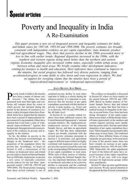
Figure 2: ‘Divergence’ of Per Capita Expenditure Across States, 1993-94 to 1999-00Average annual growth (per cent)6420BIORMPUPASKA200 300 400 500 600Source: Authors’ calculations using unit record data from the 50th and 55th Rounds of the National SampleSurvey.AI = All India; AP = Andhra Pradesh; AS = Assam; BI = Bihar; DE = Delhi; GU = Gujarat; HA = Haryana;HP = Himachal Pradesh; JK = Jammu and Kashmir; KA = Karnataka; KE = Kerala; MA = Maharashtra;MP = Madhya Pradesh; OR = Orissa; PU = Punjab; RA = Rajasthan; TN = Tamil Nadu; UP = Uttar Pradesh;WB = West Bengal.BIMARU states (Bihar, Madhya Pradesh,Rajasthan and Uttar Pradesh), and AndhraPradesh. The high-growth states, for theirpart, consist of the southern states (exceptAndhra Pradesh), the western states(Gujarat and Maharashtra) and the northwesternregion (Punjab, Haryana andHimachal Pradesh). Further, it is interestingto note that this pattern is reasonablyconsistent with independent data on growthrates of per capita ‘state domestic product’(SDP); these are shown in the last columnof Table 3. With a couple of exceptionson each side, all the states in the ‘lowAPCE growth’ set had comparatively lowrates of per capita SDP between 1993-94and 1999-2000 (say below 4 per cent peryear), and conversely, all the states in the‘high APCE growth’ set had comparativelyhigh annual growth rates of percapita SDP (the correlation coefficientbetween the two series is 0.45). 19This broad regional pattern is a matterof concern, because the low-growth statesalso tend to be states that started off withcomparatively low levels of APCE or percapitaSDP. In other words, there has beena growing ‘divergence’ of per capita expenditure(and also of per capita SDP)AIAPWBTNMAGURAHPHAKEJKPUGeometric mean PCE in 1993-94, rupees per headDEacross Indian states in the nineties. 20 Thepoint is illustrated in Figure 2, which plotsthe average growth in APCE for each statebetween 1993-94 and 1999-2000 againstthe geometric mean of APCE in 1993-94.It is worth asking to what extent theseregional patterns, based on APCE data, arecorroborated by regional patterns of povertydecline. One difficulty here is thatthere is no obvious way of ‘comparing’ theextent of poverty decline across states. Forinstance, looking at absolute changes in(say) HCRs would seem to give an unfair‘advantage’ to states that start off withhigh levels of poverty, and where theretends be a large number of householdsclose to the poverty line. To illustrate, theabsolute decline of the rural HCR between1993-94 and 1999-2000 was about twiceas large in Bihar (7.4 percentage points)as in Punjab (3.8 points), yet over the sameperiod APCE grew by only 6.9 per centin Bihar compared with 20.2 per centin Punjab, with virtually no change indistribution in either case. 21 The reasonfor this contrast is that Bihar starts off in1993-94 with a very high proportion ofhouseholds close to the poverty line, sothat small increases in APCE can producerelatively large absolute declines in theheadcount ratio.An alternative approach is to look atproportionate changes in HCRs or PGIs.These turn out to be highly correlated withthe corresponding growth rates of APCE.The point is illustrated in Figure 3, wherewe plot the proportionate decline in therural headcount ratio in each state againstthe growth rate of APCE in rural areas. Thecorrelation coefficient between the twoseries is as high as 0.91. This reflects thefact that poverty reduction is overwhelminglydriven by the growth rate of APCE,rather than by changes in distribution – weshall return to this point in Section III.From these observations, it follows that ifwe accept ‘proportionate change in HCR’(or PGI) as an index of poverty reduction,then the broad regional patterns identifiedearlier for the growth rate of APCE alsotend to apply to poverty reduction. Inparticular: (1) most of the western andsouthern states (with the important exceptionof Andhra Pradesh) have done comparativelywell; (2) the eastern region hasachieved very little poverty reductionbetween 1993-94 and 1999-2000; and(3) there is a strong overall pattern of ‘divergence’(states that were poorer to startwith had lower rates of poverty reduction).This reading of the evidence, however,remains somewhat tentative, since there isno compelling reason to accept the proportionatedecline in HCR (or PGI) as adefinitive measure of poverty decline.We end this section with a caveat. FromTable 2 and Figure 1, it may appear thatthe ‘pace’ of poverty decline in the ninetieshas been fairly rapid. It is important tonote, however, that the associated increasesin per capita expenditure have been rathermodest in most cases. For instance, thedecline of 6.6 percentage points in the all-India HCR (from 29.2 per cent to 22.7 percent) between 1993-94 and 1999-2000 isdriven by an increase of only 10.9 per centin average per capita expenditure – notexactly a spectacular improvement inliving standards. Similarly, Table 2a suggeststhat Bihar achieved a large step inpoverty reduction in the nineties, with therural HCR coming down from 49 per centto 41 per cent. Yet, as Table 3 indicates,average APCE in rural Bihar increasedby only 7 per cent between 1993-94 and1999-2000.Why are small increases in APCE associatedwith substantial declines in povertyindexes? It is tempting to answer that thedistribution of consumer expenditureEconomic and Political Weekly September 7, 2002 3735

must have improved in the nineties. Asdiscussed in Section III, however, this isnot the case: indeed economic inequalityhas increased rather than decreased in thenineties. The correct answer relates to the‘density effect’ mentioned earlier (seeSection I.2): when many poor householdsare close to the poverty line, modest increasesin APCE can produce substantialdeclines in standard poverty indexes. Onereason for drawing attention to this is thatthe official poverty estimates have sometimesbeen used to claim that the ninetieshave been a period of spectacular achievementsin poverty reduction. In fact, whenthe relevant adjustments are made, andthe poverty indexes are read together withthe information on APCE growth, povertyreduction in the nineties appears to bemore or less in line with previous rates ofprogress.IIFurther EvidenceII.1 National Accounts StatisticsThere has been much discussion of theconsistency between National SampleSurvey data and the ‘national accounts’published by the Central StatisticalOrganisation (CSO). 22 The latter includeestimates of ‘private final consumer expenditure’,which is frequently comparedwith NSS estimates of ‘household(Rural)consumption expenditure’. Over time, theCSO estimates have tended to grow fasterthan the NSS estimates, leading some commentatorsto question the reliability ofNational Sample Survey data.It is important to note that these twonotions of ‘consumer expenditure’ are notTable 3: Growth Rates of APCE and Per Capita SDP, 1993-94 to 1999-2000Six-Year Growth of APCE (‘Adjusted’), 1993-94 to 1999-2000 Annual Growth Rate ofRural Urban Combined Per Capita SDP,1993-94 to 1999-2000Assam 0.9 8.8 1.7 0.58Orissa 1.4 –0.0 3.3 2.34West Bengal 2.1 11.5 3.3 5.48Jammu and Kashmir 5.4 8.0 5.3 2.49Bihar 6.9 4.8 7.1 2.10Madhya Pradesh 6.6 14.1 7.8 2.78Andhra Pradesh 2.8 18.5 8.3 3.57Rajasthan 7.0 15.4 8.6 4.60Uttar Pradesh 8.3 10.1 9.0 2.99India 8.7 16.6 10.9 4.36Karnataka 9.5 26.5 14.0 5.82Maharashtra 14.1 16.7 15.9 3.53Gujarat 15.1 20.9 16.8 4.88Himachal Pradesh 16.2 28.5 17.6 5.06Tamil Nadu 15.7 25.1 18.9 5.39Kerala 19.6 18.2 19.6 4.01Punjab 20.2 17.9 19.9 2.74Haryana 31.0 23.0 29.2 3.05Delhi – 30.7 30.7 5.69Note: The states are arranged in ascending order of the growth rate of APCE for rural and urban areacombined.Sources: For APCE: Authors’ calculations from unit record data for the 50th and 55th Rounds of the NationalSample Survey. For SDP: Authors’ calculations based on unpublished data kindly supplied by thePlanning Commission. The figures in the last column should be taken as indicative, given thesignificant margin of error involved in SDP estimates.Proportionate decline in rural headcount ratio706050403020100–10Figure 3: HCR Declines and APCE Growth, 1993-94 to 1999-2000ASWBORAP0 5 10 15 20 25 30Source: Tables 2a and 3.JKRA UPINDIABI KAMPGUMAHPTNSix-year growth of rural APCEKEPUHAexactly the same, and also that there aremajor methodological differences betweenthe two sources. The NSS figures are directestimates of household consumption expenditure.The CSO figures include severalitems of expenditure that are notcollected in the NSS surveys; examples areexpenditures by non-profit entreprises, aswell as imputed rent by owner occupiersand ‘financial intermediation servicesindirectly measured’ (the last item is essentiallythe net interest earned by financialintermediaries, which is counted asexpenditures on intermediation servicesby households). According to Sundaramand Tendulkar (2002), who quote a recentcross-validation study by the NationalAccounts Department, the last two itemsaccount for 22 per cent of the differencein levels between CSO and NSS estimatesof consumer expenditure. Further, the CSOestimates are ‘residual’ figures, obtainedafter subtracting other items from thenational product. Leaving aside thesecomparability issues, there is indeed a gapbetween the CSO-based and NSS-basedgrowth rates of consumer expenditure.According to CSO data, per-capita consumerexpenditure has grown at muchthe same rate as per capita GDP between1993-94 and 1999-2000 – about 3.5 percent per year in real terms. 23 The correspondingNSS-based estimate associated3736Economic and Political Weekly September 7, 2002

nineties. 28 Thus, real agricultural wageswere growing considerably faster in theeighties than in the nineties. But even thereduced growth rate of agricultural wagesin the nineties, at 2.5 per cent per year,points to significant growth of per capitaexpenditure among the poorer sections ofthe population and reinforces our earlierfindings on poverty reduction. In fact, thisreduced growth rate is a little higher thanthe growth rate of average per capitaexpenditure (1.5 per cent per year) thatsustains our estimated declines of ruralheadcount ratios and headcount indexesbetween 1993-94 and 1999-2000.The data on real wages also providesome independent corroboration of thestate-specific patterns of poverty decline.This is illustrated in Figure 5, where weplot state-specific estimates of the growthrate of real agricultural wages in the ninetiesagainst the estimated proportionatedecline in the headcount ratio (a very similarpattern applies to the poverty-gap index).Here the two main outliers are Punjab andHaryana, where the headcount ratio hasdeclined sharply without a correspondinglysharp increase in real wages (indeedwithout any such increase, in the case ofPunjab). Leaving out these two outliers,the association between the two series isremarkably close (with a correlation coefficientof 0.88).An interesting sidelight emerging fromFigure 5 is that a healthy growth of realagricultural wages appear to be a ‘sufficient’condition for substantial povertydecline in rural areas: all the states wherereal wages have grown at more than, say,2.5 per cent per year in the nineties haveexperienced a comparatively sharp reductionof the rural headcount ratio. Conversely,in states with low rates of reductionof the headcount ratio (say, 15 per centor less over six years), real wages haveinvariably grown at less than 2 per centper year. This applies in particular to theentire eastern region (Assam, Orissa, WestBengal and Bihar) and also to AndhraPradesh and Madhya Pradesh.Independent evidence on the growth ratesof real wages has recently been presentedby K Sundaram (2001a, 2001b), based onthe ‘employment-unemployment surveys’(EUS) of the National Sample Survey for1993-94 and 1999-2000. For the presentpurpose, these surveys are comparable.Sundaram estimates that the real earningsof agricultural labourers have grown atabout 2.5 per cent per year between 1993-94and 1999-2000. These are tentativeRural headcount ratio (adjusted)50403020100Figure 4: Agricultural Wages and Rural Poverty, 1999-2000ORKA0 2 3 4 5 6 7 8Real agricultural wageSource: Drèze and Sen (2002), Statistical Appendix, Table A 3, and Table 2a of this paper. The “realagricultural wage” is a three-year average ending in 1999-2000.estimates, based as they are on data for twoyears only. Yet it is reassuring to find thatthey are consistent with the AWI-basedestimates.II.3 The ‘Employment-Unemployment Surveys’The National Sample Survey’s 1993-94and 1999-2000 employment-unemploymentsurveys (EUS) also include consumerexpenditure data. These can be used forfurther scrutiny of poverty trends. Thistask has been undertaken in a recent paperby Sundaram and Tendulkar (2002). Theynote that the consumption survey in the1999-2000 EUS uses the traditional 30-day reporting period, but differs from thestandard questionnaire by only asking anabbreviated set of questions. However, theauthors find that, in those cases where thequestions have comparable coverage, themeans from the EUS, using the traditional30-day reporting period, are typically closeto those from the 30-day questionnaire inthe main consumption survey. Based onthis correspondence, they argue that the30-day questions in the main 1999-2000survey were not much distorted by theseven-day questions that were asked alongsidethem. In this version of events, themajor source of incomparability betweenthe 55th and 50th Rounds is not the contaminationof the 30-day questions, butrather the revised treatment of the lowBIMPUPASAPMAINDIATNWBGURAPUHAKEfrequency items, for which the reportingperiod was 30 days in the 50th Round and365 days in the 55th Round. As we havealready noted, the 365-day reporting periodfor these items pulls up the lower tailof the consumption distribution, and thusbiases down the headcount ratio comparedwith earlier methods. However, Sundaramand Tendulkar note that the 50th Roundcontained both 30-day and 365-day reportingperiods for the low frequency items.Hence, by recalculating the 50th Roundheadcounts using the 365-day responses,they can put the 50th and 55th Rounds ona roughly comparable basis. When they dothis, they find that, in both rural and urbansectors, they can confirm a little more thanthree-quarters of the official decline in theheadcount ratios between the two rounds[Sundaram and Tendulkar 2002:Table III.8]. These calculations are notidentical to our first-step adjustments (seeTable 1a), but they are close enough toinspire some confidence that both sets ofresults are in the right range.To sum up, the all-India poverty indexespresented earlier in this paper are broadlyconsistent with independent evidence fromthe national accounts statistics and theemployment-unemployment surveys, aswell as with related information on agriculturalwages. There is also some congruencebetween the inter-state contrastsemerging from NSS data and independentinformation on state-specific growth rates3738Economic and Political Weekly September 7, 2002

Proportionate decline in rural HCR806040200Source: See Figure 4.Figure 5: Wage Growth and Poverty Decline, 1993-94 to 1999-2000PU–4 –2 0 2 4 6 8 10Growth rate of real agricultural wageof ‘state domestic product’ and real agriculturalwages. The combined evidencefrom these different sources is fairly strong,even though each individual source hassignificant limitations.IIIEconomic Inequality in theNinetiesIII.1 Growth, Povertyand InequalityMABIMPWBAPORASIt is possible to think about povertydecline, as captured by standard povertyindexes, in terms of two distinct components:a growth component and a distributioncomponent. The growth componentreflects the increase of average percapita expenditure. The distribution componentcaptures any change that may takeplace in the distribution of per capita expenditureover households.This decomposition exercise is pursuedin Table 4, with reference to the headcountratio (very similar results apply to thepoverty-gap index). The first column repeatsthe headcount ratio for 1993-94from Table 2. The second column (labelled‘derivative with respect to growth’) showsour estimate of the percentage-point reductionin HCR associated with a distribution-neutral,1 per cent increase in APCEin the relevant state. To illustrate, in ruralAndhra Pradesh a 1 per cent increase inAPCE in 1993-94, with no change inHAUPINDIARATNKAGUKEdistribution, would have led to a declineof 0.9 percentage points in the ruralheadcount ratio. 29 This derivative dependspositively on the fraction of people whoare at or near the poverty line, which istypically larger in the poorer states. Thefigures in column 2 vary from –1.27 inrural Assam to –0.15 in urban Jammu andKashmir. Column 3 reproduces the totalpercentage growth between 1993-94 and1999-2000 from Table 3.If we multiply the second column (thederivative with respect to growth) by thethird column (the amount of growth), weget an estimate of the amount of povertyreduction that we would expect from growthalone, in the absence of any change in theshape of the distribution. This is an approximation,because the derivative is likelyto change as the headcount ratio falls. Incolumn 4, we report a more precise calculation:an estimate of what the headcountratio would have been in 1999-2000 if thedistributions of consumption in each statewere identical to those in 1993-94, but hadbeen shifted upwards by the amount ofgrowth in real per capita expenditure thatactually took place. This can be readilycalculated by reducing the 1993-94 povertylines by the amount of growth, andre-estimating the headcount ratios fromthese adjusted lines and the 1993-94 expendituredata. These hypothetical changescan then be compared with the actualreductions in the headcount ratios, shownin the final column. The differencebetween these last two columns is thechange in the headcount ratio that is attributableto changes in the shape of theconsumption distribution.It is important to note that the last twocolumns are highly correlated. The correlationcoefficients across the states are0.97 (rural) and 0.93 (urban), so that growthalone can predict much of the cross-statepattern of reduction in HCRs. Nevertheless,the estimates are far from identical. Inparticular, the all-India calculations showthat ‘growth alone’ would have reduced thepoverty rate by more than actually happened,implying that there was an increasein inequality that offset some of the effectsof growth, or put differently, that APCEgrowth among the poor was less than theaverage. These inequality effects varysomewhat from state to state and are muchweaker in rural than in urban areas. Inurban India, increasing inequality moderatedthe decline in the headcount ratio inall states except Delhi, Maharashtra, andJammu and Kashmir. In some cases, suchas urban Kerala and Madhya Pradesh, the‘moderating effect’ is pronounced, withactual rates of reduction only a little over halfthose predicted by the growth in the mean.For the urban sector as a whole (the lastrow of the table), the actual decline in theHCR is one and a half points lower (5.9versus 7.4 per cent) than would have beenthe case had growth been equally distributedwithin each state. This estimate, whichis the population-weighted average of thecorresponding numbers for each state,calculates what would have happened ifeach household in each state had experiencedthe average growth for that state. Analternative, and equally interesting, counterfactualis what would have happened if,between 1993-94 and 1999-2000, eachhousehold in the country had experiencedthe countrywide growth rate of 10.9 percent. Such a calculation yields an all-IndiaHCR of 21.4 per cent (for rural and urbanareas combined), compared with an actualall-India HCR of 22.7 per cent based onthe 55th Round. In other words, the all-India HCR in 1999-2000 was 1.3 percentagepoints higher than it would have been(with the same growth rate of APCE) inthe absence of any increase in inequality.III.2 Aspects of Rising InequalityThree aspects of rising economic inequalityin the nineties have come up sofar in our story. First, we found strongevidence of ‘divergence’ in per capitaEconomic and Political Weekly September 7, 2002 3739

consumption across states. Second, ourestimates of the growth rates of per capitaexpenditure between 1993-94 and 1999-2000 (Table 3) point to a significant increasein rural-urban inequalities at the all-India level, and also in most individualstates. Third, the decomposition exercisein the preceding section shows that risinginequality within states, particularly in theurban sector, has moderated the effects ofgrowth on poverty reduction.Table 5 provides more systematic evidenceon recent changes in consumptioninequality within each sector of each stateusing two different measures of inequality.We show the logarithm of the differenceof the arithmetic and geometric means(approximately the fraction by which thearithmetic mean exceeds the geometricmean), as well as the variance of thelogarithm of per capita expenditure.The table shows that the correction forquestionnaire design is critical for understandingwhat has been happening. (Notethat the correction for prices has no effectwithin sectors and states.) The direct useof the unit record data in the 55th Round,with no adjustment, shows a substantialreduction in inequality within the ruralsectors of most states, with little or noincrease in the urban sectors. With thecorrection, we see that within-state ruralinequality has not fallen, and that therehave been marked increases in within-stateurban inequality. We suspect that the mainreason why the unadjusted data are somisleading in this context is the changefrom 30 to 365 days in the reporting periodfor the low frequency items (durable goods,clothing and footwear, and institutionalmedical and educational expenditures). Thelonger reporting period actually reducesthe mean expenditures on those items, butbecause a much larger fraction of peoplereport something over the longer reportingperiod, the bottom tail of the consumptiondistribution is pulled up, and both inequalityand poverty are reduced. Whether 365-days are a better or worse reporting periodthan 30-days could be argued either way,but the main point here is that the 55th and50th Rounds are not comparable, and thatthe former artificially shows too littleinequality compared with the latter. Oncethe corrections are made, we see that, inaddition to increasing inequality betweenstates, there has been a marked increasein consumption inequality within theurban sector of nearly all states.Two further pieces of evidence areworth mentioning in this context. First,our findings on rising economic inequalitywithin the urban sector are consistent withrecent work by Banerjee and Piketty (2001),who use income tax records to documentvery large increases in income among thevery highest income earners. They showthat, in the 1990s, real incomes among thetop one per cent of income earners increasedby a half in real terms, while thoseof the top 1 per cent of 1 per cent increasedby a factor of three in real terms.Second, it is interesting to compare thegrowth rate of real wages for agriculturallabourers with that of public sector salaries.As we saw earlier, real agriculturalwages have grown at 2.5 per cent or soin the nineties. Public sector salaries, fortheir part, have grown at almost 5 per centper year during the same period. 30 Giventhat public-sector employees tend to bemuch better off than agricultural labourers,this can be taken as an instance of risingeconomic disparities between differentTable 5: Inequality Measuresoccupation groups. Since agriculturallabourers and public sector employeestypically reside in rural and urban areas,respectively, this finding may just beanother side of the coin of rising ruralurbandisparities. Even then, it strengthensthe evidence presented earlier onaspects of rising economic inequality inthe nineties.To sum up, except for the absence ofclear evidence of rising intra-rural inequalitywithin states, we find strong indicationsof a pervasive increase in economicinequality in the nineties. This isa new development in the Indian economy:until 1993-94, the all-India Gini coefficientsof per capita consumer expenditurein rural and urban areas were fairly stable. 31Further, it is worth noting that the rate ofincrease of economic inequality in thenineties is far from negligible. For instance,the compounding of inter-state‘divergence’ and rising rural-urbanlogAM¥logGM aVariance of Logs50th Round 55th Round 55th Round 50th Round 55th Round 55th RoundAdjustedAdjustedAndhra PradeshAssamBiharGujaratHaryanaHimachal PradeshJammu and KashmirKarnatakaKeralaMadhya PradeshMaharashtraOrissaPunjabRajasthanTamil NaduUttar PradeshWest BengalAll-India Rural0.140.050.080.100.160.130.100.120.150.130.160.100.130.120.160.130.110.140.090.070.070.090.100.100.060.100.140.100.110.100.100.070.140.100.090.110.130.060.080.110.230.140.070.120.160.120.160.120.140.100.150.120.080.140.240.100.160.170.280.220.160.210.260.220.270.180.220.200.270.230.170.230.170.130.130.180.190.170.120.180.240.180.200.180.190.140.230.180.150.210.220.110.160.180.310.240.140.220.270.220.280.210.240.180.240.210.150.24Andhra PradeshAssamBiharGujaratHaryanaHimachal PradeshJammu and KashmirKarnatakaKeralaMadhya PradeshMaharashtraOrissaPunjabRajasthanTamil NaduUttar PradeshWest BengalDelhi0.170.130.150.140.130.380.130.160.200.180.210.150.130.140.210.170.190.160.160.170.140.140.160.090.180.170.170.210.140.140.130.270.180.200.170.140.170.140.150.420.120.170.220.180.210.160.140.140.200.190.190.300.250.270.250.240.370.240.310.310.290.400.290.230.250.390.310.340.290.300.300.250.270.290.160.320.320.290.360.260.250.230.340.310.310.330.270.300.260.280.400.210.340.370.330.400.290.250.260.350.340.350.29 0.21 0.30 0.43 0.39 0.46All-India Urban 0.19 0.20 0.21 0.34 0.34 0.37All-India 0.17 0.18 0.19 0.29 0.29 0.32Note: a AM is the arithmetic mean and GM is the geometric mean: the difference in their logarithms is themean relative deviation, a measure of inequality.3740Economic and Political Weekly September 7, 2002

250.0200.0150.0100.050.0Figure 6: Food Intake for Different Per Capita Income Groups, as a Proportion(Per Cent) of Average Intake (1996-97)0.0Cereals and millets Fats and oils Sugar and Jaggery Milk and milk productsPer capita income groups (Rs/cap/month) less than 90 90-150150-300 300-600 more than 600Source: Calculated from National Nutrition Monitoring Bureau (1999), Table 6.9. The data relate to ruralareas of eight sample states.disparities produces very sharp contrastsin APCE growth between the rural sectorsof the slow-growing states and the urbansectors of the fast-growing states (Table 3).This is further compounded by the accentuationof intra-urban inequality, which isitself quite substantial, bearing in mindthat the change is measured over a shortperiod of six years (Table 5).It might be argued that a temporaryincrease in economic inequality is to beexpected in a liberalising economy, andthat this trend is likely to be short-lived.Proponents of the ‘Kuznets curve’ mayeven expect it to be reversed in due course.However, China’s experience of sharp andsustained increase in economic inequalityover a period of more than 20 years, aftermarket-oriented economic reforms wereinitiated in the late 1970s, does not inspiremuch confidence in this prognosis. 32 It is,in fact, an important pointer to the possibilityof further accentuation of economicdisparities in India in the near future.IVQualifications and ConcernsIV.1 Food ConsumptionThere have been major changes in India’sfood economy in the nineties. The eightieswere a period of healthy growth in agriculturaloutput, food production, and realagricultural wages. During the nineties,however, productivity increases sloweddown in many states. The quantity indexof agricultural production grew at a lame2 per cent per year or so. The growth ofreal agricultural wages slowed down considerably.And cereal production barelykept pace with population growth. 33The virtual stagnation of per capita cerealproduction in the nineties has been accompaniedby a gradual switch from net importsto net exports, and also by a massiveaccumulation of public stocks. Correspondingly,there has been no increase in estimatedper capita ‘net availability’ of cereals(Table 6). If anything, net availabilitydeclined a little, from a peak of about 450grams per person per day in 1990 to 420grams or so at the end of the nineties. Thisis consistent with independent evidence,from National Sample Survey data, of adecline in per capita cereal consumptionin the nineties. Between 1993-94 and 1999-2000, for instance, average cereal consumptionper capita declined from 13.5 kgper month to 12.7 kg per month in ruralareas, and from 10.6 to 10.4 kg per monthin urban areas. 34 This comparison isbased on the ‘uncorrected’ 55th Rounddata, and the ‘true’ decline may be largerstill, given the changes in questionnairedesign (Section I.1).The reduction of cereal consumption inthe nineties may seem inconsistent withthe notion that poverty has declined duringthe same period. Indeed, this pattern hasbeen widely invoked as evidence of ‘impoverishment’in the nineties. If cereal consumptionis declining, how can povertybe declining?It is worth noting, however, that thedecline of cereal consumption is not new.A similar decline took place (according toNational Sample Survey data) during theseventies and eighties, when poverty wascertainly declining. Hanchate and Dyson’s(2000) recent comparison of rural foodconsumption patterns in 1973-74 and1993-94 sheds some useful light on thismatter. As the authors show, during thisperiod per capita cereal consumption inrural areas declined quite sharply on average(from 15.8 to 13.6 kgs per personper month), but rose among the pooresthouseholds. The decline in the average isdriven by reduced consumption among thehigher expenditure groups. 35The average decline is unlikely to bedriven by changes in relative prices;indeed, there has been little change in foodprices, relative to other prices, in the interveningperiod. Instead, this pattern appearsto reflect a substitution away fromcereals to other food items as incomes rise(at least beyond a certain threshold). Theconsumption of ‘superior’ food items suchas vegetables, milk, fruit, fish and meat didrise quite sharply over the same period,across all expenditure groups. Seen in thislight, the decline of average cereal consumptionmay not be a matter of concernper se. Indeed, average cereal consumptionis inversely related to per capita incomeacross countries (e g, it is lower inChina than in India, and even lower in theUnited States), and the same applies acrossstates within India (e g, cereal consumptionis higher in Bihar or Orissa than inPunjab or Haryana).Food intake data collected by the NationalNutrition Monitoring Bureau(NNMB) shed further light on this issue.Aside from detailed information on foodintake, the NNMB surveys include roughestimates of household incomes. These areused in Figure 6 to display the relationbetween per-capita income and food intake,for different types of food. The substitutionfrom cereals towards other fooditems with rising per-capita income emergesquite clearly. 36 This pattern, if confirmed,would fit quite well with the data on changeover time. 37 It also implies that the declineof average cereal consumption in the ninetiesis not inconsistent with our earlierfindings on poverty decline. 38IV.2 Localised Impoverishmentand Hidden CostsThe overall decline of poverty in thenineties does not rule out the possibilityof impoverishment among specific regionsor social groups. That possibility, of course,is not new, but it is worth asking whetherEconomic and Political Weekly September 7, 2002 3741

6.05.04.03.02.01.00.0Figure 7:Progress of Selected Social Indicators in the 1980s and 1990s(Per Cent Per Year)5.52.52.9Increase of real Decline of infant Decline of total Decline ofagricultural wages mortality rate fertility rate illiteracy rateSource: Drèze and Sen (2002), chapter 9.1.5its scope has expanded during the lastdecade. As the economy gives greater roomto market forces, uncertainty and inequalityoften increase, possibly leading toenhanced economic insecurity among thosewho are not in a position to benefit fromthe new opportunities, or whose livelihoodsare threatened by the changes in theeconomy. The increase of economic inequalityin the nineties, noted earlier,suggests that tendencies of this kind maywell be at work in India today. Adversetrends in living standards could take severaldistinct forms, including: (1) impoverishmentamong specific regions or socialgroups, (2) heightened uncertainty ingeneral, and (3) growing ‘hidden costs’ ofeconomic development.In connection with the first point, wehave already noted that some of the poorerstates, notably Orissa and Assam, have notfared well at all in the nineties. It is quitepossible that the poorer regions withinthese states have done even worse, to thepoint of absolute impoverishment forsubstantial sections of the population. Inthe case of Orissa, there is some independentevidence of localised impoverishmentin the poorer districts, due inter alia to thedestruction of the local environmental baseand to the dismal failure of state-sponsoreddevelopment programmes [Drèze2001]. 39Similarly, the overall improvement ofliving standards may hide instances ofimpoverishment among specific occupationgroups. The nineties have been a periodof rapid structural change in the Indianeconomy, leading in some cases to1.71.81.52.81980s1990sconsiderable disruption of earlier livelihoodpatterns. Examples include a deeprecession in the powerloom sector, a seriouscrisis in the edible oil industry afterimport tariffs were slashed, periodic wavesof bankruptcy among cotton growers, thedisplacement of traditional fishing bycommercial shrimp farms, and a numberof sectoral crises associated with the abruptlifting of quantitative restrictions on importsin mid-2001. 40 The destruction oflocal environmental resources is anothercommon cause of disrupted livelihoods inmany areas.A related issue is the possibility of ‘hiddenhardships’ associated with recent patternsof economic development. To illustrate,there is much evidence that, in many ofthe poorer regions of India, further impoverishmenthas been avoided mainly throughseasonal labour migration. 41 The latteroften entails significant social costs thatTable 6: Cereal Availability in the Nineties(Grams per person per day)are poorly captured, if at all, in standardpoverty indexes or for that matter in theother social indicators examined in thispaper. Examples of such costs includeirregular school attendance, the spread ofHIV/AIDS, the disruption of family life,and rising urban congestion. 42 Similarly,involuntary displacement of persons affectedby large development projects suchas dams and mines tends to have enormoushuman costs. These, again, are largelyhidden from view in income-based analysesof poverty. In fact, the incomes ofdisplaced persons often rise (with ‘cashcompensation’) even as their lives are beingshattered. 43 The ‘informalisation’ of labourmarkets is another example of economicchange with substantial hidden costs (e g,longer working hours, higher insecurity,lower status, and deteriorating work conditions).44 These issues are not new, butit is important to acknowledge the possibilitythat the hidden costs of economicgrowth have intensified in the nineties.This acknowledgement helps to reconcilethe survey-based evidence reviewedearlier with widespread media reports, inrecent years, of sectoral economic crisesand localised impoverishment. 45 Thisissue calls for further scrutiny, based onmore focused analysis of survey data aswell as on micro-studies.IV.3 The ‘Thin’ Rounds: AnUnresolved Puzzle?We have so far said very little about the‘thin’ rounds, and the poverty estimatesthat can be calculated from them. YetFigure 1 shows that the recent thin rounds,from the 51st through the 54th Round,generate poverty estimates that are hard toreconcile with the quinquennial ‘thick’rounds. If we were to connect up theseNet Production Net Imports Net Change in ‘Net Availability’Public Stocks (1+2-3)1985-89 422.7 2.0 -5.3 430.11990 456.9 0.3 5.0 452.11991 447.9 -1.4 0.4 446.11992 446.8 1.3 4.2 443.81993 446.4 2.5 16.6 432.31994 456.3 0.2 16.6 439.91995 448.6 -5.9 -2.3 445.11996 451.7 -6.9 -11.7 456.41997 445.5 -6.7 -4.2 443.01998 455.3 -4.7 11.0 439.61999 456.3 -5.4 25.3 425.62000 452.7 -5.2 30.7 416.8Note: All figures (except first row) are three-year averages centred at the year specified in the first column.Source: Calculated from Government of India (2002), p S-21.3742Economic and Political Weekly September 7, 2002

points with the official HCR estimates, wewould get a series in which poverty rosebetween 1993-94 and 1994-95, fell from1994-95 to the end of 1997, rose verysharply in the first half of 1998, and thenfell with extraordinary rapidity in 1999-2000. As we have seen, the official estimatefor 1999-2000 is too low, and the lastthin round, the 54th Round, ran for onlythe first six months of 1998, and maytherefore not be fully comparable withother rounds. Even so, and with due allowancefor corrections, it is very hard tointegrate the poverty estimates based onthe thin rounds with the picture that emergesfrom the thick rounds as well as from othersources surveyed in this paper.The story is further complicated by thefact that these thin rounds were run in twoversions, one of which resembled thestandard questionnaire up to and includingthe 50th Round, and one of which – theexperimental questionnaire – had differentreporting periods for different goods.Headcount ratios based on the experimentalquestionnaire (not shown in Figure 1)are lower than those from the standardquestionnaire, because the experimentalquestionnaire generated higher reports ofper capita expenditure. However, they alsoshow rising HCRs from the 52nd throughthe 54th Rounds, and the increase continuesinto the 55th Round if we use comparablereporting periods from that round.Based on the experimental questionnaire,a case could be made that the all-IndiaHCR has been rising since 1995-96 [Sen2000]. As we have seen, there are goodgrounds for distrusting the experimentalquestionnaire in the 55th Round, becauseof the juxtaposition of the seven-day recalland 30-day recall data for food-pan andtobacco. Quite likely, the ‘reconciliationeffect’ (see Section I.1) pulled down theestimates of per capita expenditure fromthe experimental questionnaire, thus exaggeratingpoverty by this count. Even so,if poverty were genuinely falling, there isno obvious explanation why the experimentalquestionnaire should show a risein poverty from 1995 through 1998.The Planning Commission has neverendorsed poverty counts from the thinrounds. In part, this has been because ofthe smaller sample sizes. The PlanningCommission needs estimates of HCRs, notjust for all-India, but for individual states,and the thin rounds are not large enough tosupport accurate estimates for some of thesmaller (of the major) states. But inadequatesample size generates variance,not bias, and in any case, the thin roundsample sizes are perfectly adequate togenerate accurate estimates for the all-India HCRs. The discrepancies in Figure 1cannot be explained by inadequatesample sizes.There are other differences between thickand thin rounds. For example, the samplingframe for the 51st, 53rd, and 54thRounds was not the census of population,but the ‘economic’ census. In the populationcensus, each household is asked ifit has a family business or enterprise, andonly such households are included in thefirst-stage sampling from the economiccensus when ‘first-stage units’ are drawnwith probability proportional to size. Thismeans that a village with few or no suchhouseholds has only a small or no chanceof being selected as a first-stage unit. Evenso, when the team reaches the village, allhouseholds are listed and have a chanceof being in the sample, so it is unclear thatthis choice of frame makes much difference.Indeed, comparison of various socioeconomicindicators (e g, literacy rates,years of schooling, landholding, or familysize) from the surveys suggests no obviousbreaks between the 51st and 53rd Roundson the one hand, and the 52nd Round(which used the population census) on theother. Conversations with NSS and PlanningCommission staff sometimes suggestthat there may be other (non-documented)differences in the sampling structure of thethin rounds. Certainly, a tabulation of thepopulation sizes of the first-stage unitsshows that the 52nd Round containedrelatively few large units compared withthe 51st, 53rd, 54th, and 55th rounds; thisis a different issue from the use of theeconomic rather than population census(both the 52nd and 55th Rounds use thelatter), and the finding suggests that thefirst-stage units in the 52nd Round wereselected differently from other rounds insome way that is not documented. Moreover,the measurement of consumption isnot the main purpose of any of these thinrounds, all of which have some otherobjective, so it is possible that consumptionis not so fully or carefully collectedas in the quinquennial rounds.In short, there are grounds for scepticismabout the validity of the thin rounds forpoverty estimation purposes, and this is allthe more so if we remember that aside fromindicating no poverty decline in the latenineties, the thin rounds also suggest thataverage per capita expenditure was stagnatingduring that period – something thatis very hard to reconcile with other evidence.Having said this, we have not beenable to identify any ‘smoking gun’ thatwould point to a specific problem with anyof these rounds and explain their apparentlyanomalous poverty estimates. Untilthat puzzle is resolved, we see the evidencefrom the thin rounds as casting a shadowof doubt over the interpretation of thepoverty estimates presented earlier in thispaper. Perhaps the thin rounds in the nextfive years will offer some useful clues.VBeyond Poverty IndexesThe decline of poverty in the nineties,as captured in the indicators examined sofar, can be seen as an example of continuedprogress during that period. Whether therate of progress has been faster or slowerthan in the eighties is difficult to say, andthe answer is likely to depend on how therate of progress is measured. There is, atany rate, no obvious pattern of “acceleration”or ‘slowdown’ in this respect.It is important to supplement the evidencereviewed so far, which essentiallyrelates to purchasing power, with otherindicators of well-being relating, for instanceto educational achievements, lifeexpectancy, nutritional levels, crime rates,and various aspects of social inequality.This broader perspective reveals that socialprogress in the nineties has followedvery diverse patterns, ranging from acceleratedprogress in some fields to slowdownand even regression in other respects.The point is illustrated in Figure 7,where simple measures of the progress ofdifferent social indicators in the ninetiesare compared with the correspondingachievements in the eighties.Elementary education provides an interestingexample of accelerated progress inthe nineties. 46 This trend is evident notonly from census data on literacy rates, butalso from National Family Health Surveydata on school participation. To illustrate,school participation among girls aged 6-14jumped from 59 per cent to 74 per centbetween 1992-93 and 1998-99. 47 The regionalpatterns are also instructive. It isparticularly interesting to note evidence ofrapid progress in Madhya Pradesh andRajasthan, demarcating them clearly fromBihar and Uttar Pradesh, the other twomembers of the so-called BIMARU set. 48There is an important pointer here to therelation between public action and socialachievements. Indeed, Madhya PradeshEconomic and Political Weekly September 7, 2002 3743

and Rajasthan are two states where therehave been many interesting initiatives inthe field of elementary education in thenineties (on the part of government as wellas non-government institutions), in contrastwith Bihar and Uttar Pradesh whereschooling matters continue to be highlyneglected. The fact the literacy rates andschool participation have surged in themore ‘active’ states is an encouragingindication of the possibility of effectivepublic intervention in this field.Turning to instances of ‘slowdown’, wehave already referred to the slackening ofthe growth rate of real agricultural wagesin the nineties. Another important exampleis the slowdown of infant mortality decline.During the eighties, India achieveda reduction of 30 per cent in the infantmortality rate – from 114 deaths per 1,000live births in 1980 to 80 per 1,000 in 1990.During the nineties, however, the infantmortality rate declined by only 12.5 percent – from 80 to 70. 49 In fact, in thesecond half of the nineties, India’s infantmortality rate has remained virtually unchanged.In some states, notably Rajasthan,the infant mortality rate has stagnated foras long as 10 years. These worrying trendshave received astonishingly little attentionin policy debates, and even in the debateon ‘poverty in the nineties’.Finally, there have also been some areasof ‘regression’ in the nineties. The increaseof economic inequality, discussedearlier, can be seen in those terms. Giventhe adverse social consequences of economicinequality (ranging from elitist biasesin public policy to the reinforcement ofother types of inequality), this accentuationof economic disparities is not a trivialmatter. Another example of adversedevelopment in the nineties is the declinein the female-male ratio among children,from 945 girls per 1,000 boys (in the 0-6age group) in 1991 to 927 girls per 1,000boys in 2001. 50 This decline appears to bedriven by the spread of prenatal sexdeterminationtechnology and sexselectiveabortion, but this does not meanthat it is a ‘technological’ phenomenon,unrelated to other recent economic andsocial trends. Economic growth, in particular,may facilitate the spread of sexselectiveabortion, by making the use ofsex-determination technology more affordable.In this connection, it is worth notingthat the largest declines of the female-maleratio among children between 1991 and2001 occurred in five states (Gujarat,Haryana, Himachal Pradesh, Punjab andDelhi) that are relatively well-off economically,and have also experienced comparativelyhigh rates of growth of per capitaexpenditure in the nineties (Table 3). 51A detailed assessment of the progress ofdevelopment indicators in the nineties isbeyond the scope of this paper. However,a few general observations can be madeon the basis of these illustrations. First, asnoted already, poverty is not unidimensional.The poverty indexes used in thefirst part of this paper are useful indicatorsof inadequate purchasing power, but ontheir own do not do justice to the rangeof deprivations we ought to be concernedwith. Following on this, it is important toacknowledge that recent progress in eliminatingpoverty and deprivation has beenquite uneven in different fields. The debateon ‘poverty in the nineties’ has oftenoverlooked this basic point.Second, this recognition is also importantin assessing the relation betweenpoverty decline and economic growth. Asnoted earlier, the decline of poverty in thenineties, as captured by conventional indexessuch as the headcount ratio or thepoverty-gap index, has been overwhelminglydriven by the growth of average percapita expenditure. From this it may seemthat the reduction of poverty is mainly aquestion of economic growth. However,there is an element of circularity in thisargument: if poverty is defined as lack ofincome, it is not surprising that the growthof income plays a key role in reducing it.When the multidimensional nature ofpoverty is acknowledged, this relationappears in a different light. To illustrate,consider child mortality as an aspect of thedeprivations associated with poverty. Thereis, of course, a significant (negative) relationbetween child mortality and purchasingpower. But child mortality is alsostrongly influenced by other factors suchas educational levels, fertility rates, publichealth provisions (including clean waterand vaccinations), and various aspects ofgender relations. Looking at inter-statecontrasts in India, the correlation betweenchild mortality and average per capitaexpenditure (or even poverty indexes) isactually quite weak. Other factors, particularlyfemale literacy, are often more important.52 Similar comments apply in thecontext of elementary education: the ninetieshave demonstrated the possibility ofrapid progress in this field through publicintervention, with or without rapid economicgrowth. In short, the standard focuson headcount ratios and other expenditurebasedpoverty indexes tends to foster asimplistic view of the relation betweeneconomic growth and poverty decline.Third, it is also interesting to re-examinethe issue of trends in inequality, in the lightof this broader perspective. As discussedin Section III, there is much evidence ofrising economic inequality in the nineties,in the form of a widening rural-urban gap,enhanced inter-state disparities, and alsogrowing inequality within urban areas inmost states. What about other types ofsocial inequality, involving other dimensionsof well-being (e g, educational levelsor life expectancy) and other bases ofdisadvantage (e g, gender or caste)? Thedecline of the female-male ratio amongchildren illustrates the fact that the phenomenonof rising inequality in the ninetiesis not confined to standard economicinequalities: ‘natality inequality’ betweenmales and females is also rising. 53 But thisis not to say that inequality has risen acrossthe board. Even within the field of genderinequality, there are changes in the otherdirection, such as the emergence of asubstantial gender gap in life expectancyin favour of women, overturning India’slong history of female disadvantage in thisrespect. Similarly, it is interesting to notethat while economic disparities betweenrural and urban areas have sharply risenin the nineties, there are trends in theopposite direction as well. The rural-urbangap in life expectancy, for instance, hasdeclined from 10 years or so in the late1970s to seven years or so today, and ruralurbandifferentials in school participationhave also narrowed. 54 Here again, thepicture is more diverse (and more interesting)than it appears on the basis ofpurchasing-power indicators alone.Fourth, the broad approach explored herecalls for a correspondingly broad readingof the causal influences underlying theidentified changes. In the debate on ‘povertyin the nineties’, there has been atendency not only to view developmenttrends in unidimensional terms, but alsoto attribute these trends in a somewhatmechanical manner to the economic reformsinitiated around 1991. At one endof the spectrum, it has been claimed thatthe last decade has been a period of unprecedentedimprovement in living standards,thanks to liberalisation. 55 At theother end, the nineties have been describedas a period of widespread ‘impoverishment’,attributed to liberalisation. 56 Clearly,these readings fail to do justice to thediversity of recent trends. But in addition,3744Economic and Political Weekly September 7, 2002

they ignore the diversity of causal influencesthat have a bearing on these trends.The accelerated progress of elementaryeducation in the nineties, for instance, haslittle to do with liberalisation, and the sameapplies to the slowdown of infant mortalitydecline, not to speak of the decline ofthe female-male ratio among children.Much else than liberalisation has happenedin the nineties, and while issues of economicreform are of course extremelyimportant, so are other aspects of economicand social policy.VIConcluding RemarksA number of useful lessons emerge fromthis reexamination of the evidence onpoverty and inequality in the nineties. First,there is consistent evidence of continuingpoverty decline in the nineties, in terms ofthe ‘headcount ratio’. The extent of thedecline, however, remains somewhatuncertain at this time. Given the methodologicalchanges that took place betweenthe 50th and 55th Rounds of the NationalSample Survey, the official figures (implyinga decline from 36 per cent to 26 percent in the all-India headcount ratio between1993-94 and 1999-2000) are, strictlyspeaking, invalid. We have discussedalternative estimates, based on comparabledata from the two surveys. As it turns out,these adjusted estimates suggest that alarge part of the poverty decline associatedwith official figures is ‘real’, rather thandriven by methodological changes. Whilefurther corroboration and investigation ofthe adjustment procedure is required, theresults have been supported by one independentstudy using an entirely differentmethodology [Sundaram and Tendulkar2002]. Further, the adjusted figures fitreasonably well with related evidence fromthe national accounts statistics, the employment-unemploymentsurveys, and dataon agricultural wages.Second, we have discussed some importantlimitations of the headcount ratio asan index of poverty (even within the standardexpenditure-based approach), andargued for wider adoption of alternativepoverty indexes such as the poverty-gapindex. The main argument for usingheadcount ratios is that they have good‘communication value’, in so far as theyare relatively easy to understand and interpret.However, this transparency is tosome extent deceptive, and much cautionis required in interpreting poverty trendson the basis of headcount ratios. For thepurpose of the poverty comparisons examinedin this paper, the headcount ratio turnsout to be no less informative than thepoverty-gap index. Yet it was importantto calculate the PGIs, if only to discoverthat this refinement does not, after all,make much difference in this particularcontext.Third, growth patterns in the nineties arecharacterised by major regional imbalances.Broadly speaking, the western and southernstates (Andhra Pradesh excluded) havetended to do comparatively well. The lowgrowth states, for their part, form a largecontiguous region in the north and east.This is a matter of concern, since thenorthern and eastern regions were poorerto start with. Indeed, National SampleSurvey data suggest a strong pattern ofinter-regional ‘divergence’ in average percapita expenditure (APCE): states thatstarted off with higher APCE levels alsohad higher growth rates of APCE between1993-94 and 1999-2000. In some of thepoorer states, notably Assam and Orissa,there has been virtually zero growth ofaverage per capita expenditure (and verylittle reduction, if any, in rural poverty)between 1993-94 and 1999-2000. Theseregional patterns are at least broadly consistentwith independent estimates of thegrowth rates of state domestic product(SDP).Fourth, the intensification of regionaldisparities is only one aspect of a broaderpattern of increasing economic inequalityin the nineties. Two other aspects are risingrural-urban disparities in per capita expenditure,and rising inequality of per capitaexpenditure within urban areas in moststates. Further, the real wages of agriculturallabourers have increased more slowlythan per capita GDP, and conversely withpublic sector employees, suggesting someintensification of economic inequalitybetween occupation groups.Fifth, we have argued for assessingchanges in living standards in a broaderperspective, going beyond the standardfocus on expenditure-based indicators. Inthat broader perspective, a more diversepicture emerges, with areas of acceleratedprogress in the nineties as well as slowdownin other fields. For instance, thereis much evidence of rapid progress in thefield of elementary education, but the rateof decline of infant mortality has sloweddown. These and related trends deservegreater attention than they have received sofar in the debate on ‘poverty in the nineties’.Sixth, the case for going beyond expenditure-basedindicators applies also to theassessment of inequality. While expenditure-baseddata suggest rising disparitiesin the nineties, the same need not applyto other social indicators. For instance,while economic disparities between ruraland urban areas have increased in thenineties, there has been some narrowingof the rural-urban gap in terms of lifeexpectancy and school participation.Finally, we have argued against readingthese trends simply as evidence of theimpact (positive or negative) of ‘liberalisation’.For one thing, the impact of liberalisationis a ‘counterfactual’ question, andmuch depends on how the alternatives arespecified. For another, much else has happenedin the nineties, other than liberalisation.The evidence we have reviewed isof much interest in its own right, independentlyof the liberalisation debate. Muchwork remains to be done in terms of identifyingthe causal relations underlying thetrends we have identified. EPWNotes[We are grateful to Suresh Tendulkar for helpfulcomments]1 See Datt (1999a), Gupta (1999), Bhalla (2000a,2000b), Deaton and Tarozzi (2000), Drèze(2000), Lal, Mohan and Natarajan (2001),Nagaraj (2000), Ravallion (2000), Sen (2000),Sundaram and Tendulkar (2000, 2001, 2002),Visaria (2000), Sundaram (2001a, 2001b,2001c), Chandrasekhar and Ghosh (2002),Datt and Ravallion (2002), among others.2 On the first position, see, e g, Bhalla (2000a),Bhagwati (2001), Das (2000). On the otherside, see Mehta (2001), Sainath (2001a,2001b), Shiva (2001a), among others.3 These estimates build on earlier work by Deatonand Tarozzi (2000), Deaton (2001a, 2001b)and Tarozzi (2001).4 In the 50th Round, the correlation between thelogarithm of total household per capitaexpenditure and the logarithm of per capitaexpenditure on this subset of commodities is0.79 and 0.86 in the rural and urban sectors,respectively.5 More precisely, and somewhat less restrictively,we require that the probability of beingpoor, given the amount of a household’sexpenditure on these intermediate goods,remains the same in the 55th Round as it wasin the 50th. We require this on a state by statebasis, one sector at a time, which allows theconditional probability to vary by state and bysector.6 In Deaton and Tarozzi (2000), it is shown that,between the 43rd and 50th Rounds, thecomponent of the CPIAL for the uncovereditems grew somewhat less rapidly than thecomponent for the covered items. In consequence,if we were to supplement our priceindexes for uncovered items from the CPIAL,Economic and Political Weekly September 7, 2002 3745

the estimated rate of increase of consumerprices would come down, and correspondingly,there would be a faster decline in the povertyindexes, at least for the period falling betweenthese two rounds (i e, 1987-88 to 1993-94).7 The Törnqvist price index is a weightedgeometric index with weights that are theaverage of the expenditure shares in the baseand comparison periods. It is a superlativeindex in the sense of Diewert (1976).8 For further details, see EPW ResearchFoundation (1993). On the conceptual andpractical problems involved in defining ‘calorienorms’, see Dasgupta and Ray (1990) andOsmani (1990), and the literature cited there.Note also that, if the calorie norms were tobe reapplied today, they would not generatethe same poverty lines. Updating calorie-normbased poverty lines for inflation does notpreserve their calorie-norm status.9 Similar issues arise, of course, in the contextof inter-state comparisons, especially betweenstates (e g, Kerala and Uttar Pradesh) withradically different consumption patterns andsocial environments. In both cases, comparisonsof living standards call for supplementingexpenditure data with other types ofinformation, relating for instance to publicamenities, health achievements, educationallevels, etc.10 The official line is actually 115.20. We use115.70 because this is the figure yielded bythe official methodology when the calculationsare based on the unit record data, as opposedto the interpolations used by the PlanningCommission. See notes to Table 2.11 The case of Delhi is handled differently.Because there are few sample households inrural Delhi, it is not advisable to use the priceindex for rural Delhi as part of the calculations.The poverty line for urban Delhi is calculatedfrom the all-India urban poverty line bymultiplying it by the price index for urbanDelhi relative to urban India.12 Note that this is not the only way of using theindexes; another (but only one other) possibilitywould be to update the poverty line for eachsector of each state by its own inflation rate.Because we are dealing with price indexes, notprices, the different alternatives will givedifferent answers.13 More precisely, the poverty-gap index (PGI)calculates the total shortfall of consumptionbelow the poverty line, per capita of the totalpopulation, and expressed as a percentage ofthe poverty line: PGI ≡ (1/z)[(Σ (z-y i)/n] wherez is the poverty line, n is the population size,and y iis the consumption level of the ith poorperson.14 The poverty-gap index, however, retains onelimitation of the headcount ratio: it is notsensitive to the distribution of per capita expenditurebelow the poverty line. This limitationis overcome by higher-order members ofthe FGT class, such as the ‘squared povertygapindex’ (SPGI), and also by the Sen index.While we have calculated the SPGI estimates,we confine ourselves here to the poverty-gapindex, for two reasons. First, it is easier tointerpret. Second, SPGIs are highly sensitiveto measurement errors at the bottom of the percapita expenditure scale, and their reliabilitycalls for further scrutiny.15 See Government of India (1993b), p 16.16 In Table 2 and elsewhere in this paper, theterms ‘Bihar’, ‘Madhya Pradesh’ and ‘UttarPradesh’ refer to these states as they existedprior to the formation of Jharkhand, Chattisgarhand Uttaranchal in late 2000.17 In the first sub-period, the estimates suggestsome increase in poverty in rural Haryanaand Himachal Pradesh, and also in urbanHimachal Pradesh, Punjab and Delhi. Thesepatterns, however, should be interpreted withcaution, given the relatively small samplesizes for these states and the possibility oftransient fluctuations in poverty levels inspecific years.18 Here and elsewhere, it is useful to rememberthat the period between 1993-94 and 1999-2000 was one of ‘peak’ economic growthfor the Indian economy, with per capitaGDP growing at a healthy 4.4 per cent peryear.19 While the relative growth rates of APCE indifferent states are consistent with thecorresponding relative growth rates of percapita SDP, the levels of per capita SDP growthtend to be higher than those of APCE growth.We shall return to this issue in the next section,with reference to the all-India figures.20 On the growing divergence of per capita SDPin the nineties, see also Ahluwalia (2000) andDrèze and Sen (2002).21 For inequality indexes, see Table 5 inSection III.22 See particularly Bhalla (2000a), Kulsheshtraand Kar (2002), Ravallion (2000), Sen (2000),Sundaram and Tendulkar (2001).23 Calculated from Central Statistical Organisation(2001), p xxxii.24 In nominal terms, between 1993-94 and 1999-2000, consumer expenditure has been growingat about 11.5 per cent per year according toCSO data, and 10 per cent per year accordingto our NSS-based estimates. Both the CSO’simplicit price deflator and our Törnqvist indexhave been growing at 8 per cent per year orso during this period. Thus, differences inprice deflators do not seem to help to resolvethe CSO-NSS discrepancy in this case, eventhough price-index differences may haveplayed a role in enhancing that discrepancyin earlier periods (see Sen, 2000).25 The NSS surveys, for their part, almost certainlydisproportionately miss wealthy households atthe very top of the distribution, and as Banerjeeand Piketty (2001) have shown, there has beena marked rise in incomes among the veryhighest earners. Even so, they show that thetotal amount of these earnings is not enoughto explain the increasing disparity between theNSS and the CSO estimates of consumptionexpenditure.26 For details, see, e g, Acharya (1989).27 See, e g, Jose (1988) and Sarmah (2000). Notethat the ‘real wage’ estimates used here ignoreinter-state differences in price levels.28 See Drèze and Sen (2002), p 328; on theslowdown of the growth rate of real agriculturalwages in the nineties (compared with theeighties), see also Sarmah (2000, 2001).29 Note that these derivatives are not elasticitiesin the usual sense, and are not the same asthe elasticities sometimes quoted, which arethe derivatives of the logarithm of the headcountratio with respect to the logarithm of mean percapita expenditure.30 Calculated from Government of India (2002),p S-51. There have been further major increasesin public sector salaries after 1999-2000, withthe gradual implementation of the recommendationsof the Fifth Pay Commission bymany state governments.31 See Drèze and Sen (2002), Statistical Appendix,Table A.6; also Datt (1999a, 1999b).32 On rising income inequality in China in thepost-reform period, see Bramall and Jones(1993), Griffin and Zhao Renwei (1993), YaoShujie (1999), Khan and Riskin (2001), amongothers.33 On these and related trends, see Drèze and Sen(2002), chapter 9. On the growth of foodgrainproduction, see Government of India (2002),pp S-21 and S-22.34 See Shariff and Mallick (1999), Table 5, andNational Sample Survey Organisation (2001),pp A-101 and A-134.35 For similar observations based on a comparisonof 1972-73 and 1993-94 NSS data, see Rao(2000).36 For further evidence, see also National Instituteof Nutrition (1997). This pattern, sometimesknown as the ‘nutrition transition’, is familiarto nutritionists [Drewnoski 1999]. It is worthnoting that its implications for health are notuncontroversial; some nutrition experts haveapparently “pointed to the beneficial healtheffects of dire poverty, poor diets, and strenuousmanual labour”, presumably referring to thebenefits of a low fat, low sugar, and high fibrediet, rather than low quantities. (Drewnoski,1999, p 195).37 Unlike NNMB data, National Sample Surveydata suggest that per capita cereal consumptionrises monotonically with per capita expenditure.The contradiction between nutritionalfood intake and expenditure surveys is neitheruncommon nor fully understood; for twodifferent interpretations of the Indian case, seeSubramanian and Deaton (1996) andSubramanian (2001).38 Also worth noting in this context is tentativeevidence of recent improvement in nutritionalindicators based on anthropometricmeasurements. According to NNMB data, theproportion of adults with a low “body massindex” has declined in the nineties [seeVaidyanathan 2002]. The National FamilyHealth Surveys also suggest that the proportionof undernourished children has declinedbetween 1992-93 and 1998-99 [see InternationalInstitute for Population Sciences 1995:xxxiii, and International Institute for PopulationSciences, 2000: 267 and 443].39 It should also be noted, however, that Orissawas hit by a devastating cyclone in October1999, around the middle of the 55th Roundsurvey period. The 1999-2000 povertyestimates for Orissa are therefore likely to besomewhat ‘above trend’.40 For insightful case studies of localisedeconomic crises in the nineties, see e g, Roy(1999), Breman (2001a), Krishna (2001),Jhabvala and Sinha (2002), Samal (2002), andDabir-Alai (2002).41 See Rodgers and Rodgers (2000), Rogaly etal. (2001), Sharma (2001), Institute for HumanDevelopment (2002), among others.3746Economic and Political Weekly September 7, 2002

42 On the other hand, labour migration canalso have positive roles, such as facilitatingthe diffusion of knowledge [Maharatna 2001]and enabling the disadvantaged castes to“escape from the clutches of the prevailingcaste discrimination in the village” [Sharma2001: 18].43 For a telling case study of the human costsof involuntary displacement, see Bhatia (1997).44 On this, see particularly Breman (2001a,2001b).45 See e g, Sainath (2001a, 2001b, 2001c, 2001d),Breman (2001b), Drèze (2001), Mehta (2001).We are not referring here to media reports ofshort-term hardship associated with the recentdrought (in 2000 and 2001), but to stories ofsustained impoverishment.46 For further discussion, see Drèze and Sen(2002), chapter 5.47 See Drèze and Sen (2002), p 148; alsoInternational Institute for Population Sciences(1995, 2000), for further details.48 To illustrate, looking at the percentagereduction in illiteracy between 1991 and 2001,Madhya Pradesh and Rajasthan did better thanany other major state except Himachal Pradesh;Uttar Pradesh is very close to the all-Indiaaverage; and Bihar ranks second from thebottom (calculated from census data given inGovernment of India, 2001b). The comparisonis particularly instructive because all fourBIMARU states started off with similar (verylow) levels of literacy in 1991. On the ‘schoolingrevolution’ in Himachal Pradesh (an even moreremarkable example of successful promotionof elementary education), see PROBE Team(1999), chapter 9.49 See Government of India (1999a), Table 1,and Sample Registration Bulletin, April 2001;also UNICEF (2001) and Mari Bhat (2002).The comparison with Bangladesh is alsoinstructive: Bangladesh’s infant mortality ratewas much higher than India’s in 1990 (91 and80 per 1,000, respectively), but by 1999 it hadcome down to 61 as against India’s 71. SeeWorld Development Indicators 2001, pp 16-17.50 On this and related issues, see Drèze and Sen(2002), chapter 7.51 The relevant female-male ratios are given inGovernment of India (2001b), pp 92-94.52 Across states, the correlation coefficient betweenchild mortality and per capita expenditureis 0.4 (in absolute value), compared with 0.8for the correlation coefficient between childmortality and female literacy. After controllingfor female literacy, per capita expenditurebears no significant association with childmortality at the state level. For further discussion,see Drèze and Sen (2002), pp 87-89.On the determinants of mortality and fertilityin India, see also Murthi, Guio and Drèze(1995) and Drèze and Murthi (2001), andfurther studies cited there.53 On ‘natality inequality’ and its significance,see Sen (2001).54 See e g, Government of India (1999), p 16,and Drèze and Sen (2002), p 148.55 To illustrate: “Economic reforms initiated in1991 have led to a radical transformation inthe well-being of the bottom half of the population.From an approximate level of 38 per centin 1987, poverty level in India in 1998 wasclose to 12 per cent” [Bhalla 2000b, p 7].56 To illustrate: “Both under the World Bankstructural adjustment, and from the financeministry – it’s feet might be in India, but it’shead is in Washington – and then under theWorld Trade Organisation obligations, we’rebasically getting a fundamental destruction ofnotions of the rights of citizens… Very vitalresources we need both for survival – drinkingwater, all the resources people need forlivelihoods – are just disappearing so rapidlythat life is becoming impossible…we reallyhave a very, very major crisis of survival athand....” [Shiva 2001b]. For further contributionson both sides of the debate, see theliterature cited in footnote 2.ReferencesAcharya, Sarthi (1989): ‘Agricultural Wages inIndia: A Disaggregated Analysis’, IndianJournal of Agricultural Economics, 44.Ahluwalia, Montek S (2000): ‘EconomicPerformance of States in Post-reforms Period’,Economic and Political Weekly, May 6.Banerjee, A and Piketty, T (2001): ‘Are the RichGrowing Richer: Evidence from Indian TaxData’, MIT, Cambridge MA, and CEPREMAP,Paris, processed. Available at http://www.worldbank.org/indiapovertyworkshop.Bhagwati, Jagdish (2001): ‘Growth, Poverty andReforms’, Economic and Political Weekly,March 10.Bhalla, Surjit (2000a): ‘Growth and Poverty inIndia: Myth and Reality’, mimeo, OxusResearch and Investments, New Delhi.– (2000b): ‘FAQ’s on Poverty in India’, mimeo,Oxus Research and Investments, New Delhi.Bhatia, Bela (1997): ‘Forced Evictions in theNarmada Valley’ in Drèze, J P , Samson, M,and Singh, S (eds) (1997), The Dam and theNation: Displacement and Resettlement in theNarmada Valley, Oxford University Press,New Delhi.Bramall, Chris, and Jones, Marion (1993): ‘RuralIncome Inequality in China since 1978’,Journal of Peasant Studies, 21(1).Breman, Jan (2001a): ‘An Informalised LabourSystem: End of Labour Market Dualism’,Economic and Political Weekly, 35(52).– (2001b): ‘The State of Poverty in Urban Indiaat the Beginning of the 21st Century’,Sukhamoy Chakravarty Memorial Lecture,Delhi School of Economics, November 16.Central Statistical Organisation (2001): NationalAccounts Statistics 2001, CSO, New Delhi.Chandrasekhar, C P, and Ghosh, J (2002): TheMarket that Failed: A Decade of NeoliberalEconomic Reforms in India, Leftword Books,New Delhi.Dabir-Alai, Parviz (2002): ‘The Socio-Economicsof Street Vending: A Case Study ofVulnerability for Delhi in the 1990s’, mimeo,Richmond School of Business, London.Das, Gurcharan (2000): India Unbound, Penguin,New Delhi.Dasgupta, Partha, and Ray, Debraj (1990):‘Adapting to Undernourishment: TheBiological Evidence and Its Implications’ inDrèze and Sen (1990), vol i.Datt, Gaurav (1999a): ‘Has Poverty Declined sinceEconomic Reforms?’, Economic and PoliticalWeekly, December 11-17.– (1999b): ‘Poverty in India: Trends and Decompositions’,mimeo, World Bank, Washington,DC.Datt, Gaurav, and Ravallion, Martin (2002): ‘IsIndia’s Economic Growth Leaving the PoorBehind?’, mimeo, World Bank, Washington,DC.Deaton, Angus (2001a): ‘Adjusted Indian PovertyEstimates for 1999-2000’, Princeton, ResearchProgramme in Development Studies, processed.Available at http://www.wws.princeton.edu/~rpds.– (2001b): ‘Computing Prices and Poverty Ratesin India, 1999-2000’, Princeton, ResearchProgramme in Development Studies, processed.Available at http://www.wws.princeton.edu/~rpds.Deaton, Angus and Tarozzi, Alessandro (2000):‘Prices and Poverty in India’, Princeton, ResearchProgramme in Development Studies,processed. Available at http://www.wws.princeton.edu/~rpds.Diewert, W Erwin (1976): ‘Exact and SuperlativeIndex Numbers’, Journal of Econometrics, 4.Drewnowski, Adam (1999): ‘Fat and Sugar in theGlobal Diet: Dietary Diversity in the NutritionTransition’ in Grew, R (ed), Food in GlobalHistory, Westview, Boulder.Drèze, Jean (2000): ‘Poverty: Beyond HeadcountRatios’, The Hindu, September 9.– (2001): ‘No More Lifelines: Political Economyof Hunger in Orissa’, The Times of India,September, 17.Drèze, Jean, and Murthi, Mamta (2001): ‘Fertility,Education, and Development: Evidence fromIndia’, Population and Development Review,27.Drèze, Jean and Sen, Amartya (eds) (1990): ThePolitical Economy of Hunger, Clarendon,Oxford.– (2002): India: Development and ParticipationOxford University Press, New Delhi.EPW Research Foundation (1993): ‘Poverty Levelsin India: Norms, Estimates and Trends’,Economic and Political Weekly, August 21.Government of India (1993a): Report of the ExpertGroup on Estimation of Proportion andNumber of Poor, Planning Commission, NewDelhi.– (1993b): Sample Registration System: Fertilityand Mortality Indicators 1990, Office of theRegistrar General, New Delhi.– (1999): Compendium of India’s Fertility andMortality Indicators 1971-1997, Office of theRegistrar General, New Delhi.– (2001a): Economic Survey 2000-2001, Ministryof Finance, New Delhi.– (2001b): ‘Provisional Population Totals’, Censusof India 2001, Series 1(India), Paper 1 of 2001,Office of the Registrar General, New Delhi.–(2002): Economic Survey 2001-2002, Ministryof Finance, New Delhi.Griffin, K, and Zhao Renwei (eds) (1993): TheDistribution of Income in China, Macmillan,London.Gupta, S P (1999): ‘Tricle Down Theory Revisited:The Role of Employment and Poverty’, V BSingh Memorial Lecture, 41st Annual Conferenceof the Indian Society of LabourEconomics, November 18-20, Mumbai.Hanchate, A and Dyson, T (2000): ‘Trends in theComposition of Food Consumption and theirImpact on Nutrition and Poverty in India’,mimeo, London School of Economics.Economic and Political Weekly September 7, 2002 3747

Institute for Human Development (2002):‘Dynamics of Poverty, Employment andHuman Development in Bihar’, project report;to be published as a monograph.International Institute for Population Sciences(1995): National Family Health Survey1992-93: India, IIPS, Mumbai.– (2000): National Family Health Survey 1998-99(NFHS-2): India, IIPS, Mumbai.Jhabvala, R and Sinha, S (2002): ‘Liberalisationand the Woman Worker’, Economic andPolitical Weekly, May 25.Jose, A V (1988): ‘Agricultural Wages in India’,Economic and Political Weekly, June, 25.Khan, A R and Riskin, C (2001): Inequality andPoverty in China in the Age of Globalisation,Oxford University Press, New York.Krishna, Sridhar (2001): ‘Phasing Out of ImportLicensing: Impact on Small-scale Industries’,Economic and Political Weekly, July 7.Kulshreshtha, A C and Kar, A (2002): ‘Estimatesof Food Consumption Expenditure fromHousehold Surveys and National Accounts’,paper presented at the joint Planning Commission/WorldBank workshop on povertymeasurement, Delhi, January. Available athttp://www.worldbank.org/indiapovertyworkshop.Lal, D, Mohan, R and Natarajan, I (2001):‘Economic Reforms and Poverty Alleviation:A Tale of Two Surveys’, Economic andPolitical Weekly, March, 24.Maharatna, Arup (2001): ‘On the ‘Brighter Side’of Seasonal Migration: A Case Study of FertilityTransition in Tribal Population in RuralWest Bengal, India’, mimeo, Gokhale Instituteof Politics and Economics, Pune.Mari Bhat, P N (2002): ‘Has the Decline in InfantMortality Rate Slowed Down? A Review ofSRS Evidence’, paper presented at a nationalworkshop on ‘Infant Mortality: Levels, Trendsand Interventions’ held at New Delhi onApril 11-12.Mehta, Jaya (2001): ‘Give Poverty a Face Please!’,in Alternative Economic Survey 2000-2001,Rainbow Publishers, Delhi.Murthi, M, Guio, A C and Drèze, J P (1995):‘Mortality, Fertility and Gender Bias in India’,Population and Development Review, 21.Nagaraj, R (2000): ‘Indian Economy since 1980:Virtuous Growth or Polarisation?’, Economicand Political Weekly, August 5.National Institute of Nutrition (1997): 25 Yearsof National Nutrition Monitoring Bureau, NIN,Hyderabad.National Nutrition Monitoring Bureau (1999):Report of Second Repeat Survey – Rural(1996- 97), National Institute of Nutrition,Hyderabad.National Sample Survey Organisation (2001a):‘Level and Pattern of Consumer Expenditurein India 1999-2000’, Report 457, NationalSample Survey Organisation, New Delhi.– (2001b): ‘Consumption of Some ImportantCommodities”, Report 461, National SampleSurvey Organisation, New Delhi.Osmani, Siddiq R (1990): ‘Nutrition and theEconomics of Food: Implications of SomeRecent Controversies’ in Drèze and Sen (1990),vol i.PROBE Team (1999): Public Report onBasic Education in India, Oxford UniversityPress, New Delhi.Rao, C H Hanumantha (2000): ‘Declining Demandfor Foodgrains in Rural India: Causes andImplications’, Economic and Political Weekly,January 22.Ravallion, Martin (2000): ‘Should PovertyMeasures be Anchored to the NationalAccounts?’, mimeo, ARQADE, University ofToulouse.Rodgers, Gerry and Rodgers, Janine (2000): ‘Semi-Feudalism Meets the Market: A Report fromPurnia’, Working Paper 6, Institute for HumanDevelopment, New Delhi.Rogaly, B, Biswas, J, Coppard, D, Rafique,A, Rana, K and Sengupta, A (2001): ‘SeasonalMigration, Social Change and Migrants’ Rights:Lessons from West Bengal’, Economic andPolitical Weekly, December 8.Roy, Tirthankar (1999): ‘Growth and Recessionin Small-Scale Industry: A Study of TamilNadu Powerlooms’, Economic and PoliticalWeekly, October 30.Sainath, P (2001a): ‘Will the Real NationalCalamity Please Stand Up?’, The Hindu,February 25.– (2001b): ‘It’s the Policy, Stupid, Not Implementation’(2 parts), The Hindu, September.– (2001c): ‘Mass Media: Disconnected from MassReality’, The Hindu, September 2.– (2001d): ‘Where Stomachaches Are Terminal’,The Hindu, April 29.Samal, K C (2002): ‘Shrimp Culture in ChilikaLake: Case of Occupational Displacement ofFishermen’, Economic and Political Weekly,May 4.Sarmah, Sasanka (2000): ‘Agricultural Wages:Trends and Determinants’, M Phil thesis, DelhiSchool of Economics.– (2001): ‘Agricultural Wages in India: An Analysisof Regions and States’, mimeo, Centre forDevelopment Economics at the Delhi Schoolof Economics; forthcoming in Indian Journalof Labour Economics.Sen, Abhijit (2000): ‘Estimates of ConsumerExpenditure and its Distribution’, Economicand Political Weekly, December 16.Sen, Amartya (2001): ‘Many Faces of GenderInequality’, Frontline, October 27, 2001.Shariff, A and Mallick, A C (1999): ‘Dynamicsof Food Intake and Nutrition by ExpenditureClass in India’, Economic and Political Weekly,July 3.Sharma, Alakh (2001): ‘Agrarian Relations andSocio-Economic Change in Bihar’, paperpresented at a conference on ‘Labour andCapitalist Transformation in Asia’ held at theCentre for Development Studies, Thiruvananthapuram,December 13-15.Shiva, Vandana (2001a): ‘India: Corporatisationof Agriculture Disastrous’, The Guardian,March 7.–(2001b): ‘Is Globalisation Killing the Environment?’,interview with Frederick Noronha;available at http://www.onweb.org/archive/features/shiva/shiva.html.Subramanian, A (2001): ‘Are Income-CalorieElasticities Really High in DevelopingCountries? Some Implications for Nutritionand Income’, mimeo, National Council ofApplied Economic Research, New Delhi.Subramanian, Shankar and Angus Deaton (1996):‘The Demand for Food and Calories’, Journalof Political Economy, 104, 133-62.Sundaram, K (2001a): ‘Employment-Unemployment Situation in Nineties: SomeResults from NSS 55th Round Survey’,Economic and Political Weekly, March, 17.– (2001b): ‘Employment and Poverty in 1990s:Further Results from NSS 55th RoundEmployment-Unemployment Survey, 1999-2000’, Economic and Political Weekly,August 11.– (2001c): ‘Poverty in India: Some Issues inMeasurement and Database’, mimeo, DelhiSchool of Economics, Delhi.Sundaram, K and Tendulkar, S (2000): ‘Povertyin India: An Assessment and Analysis’, draftreport for the Asia Development Bank; mimeo,Delhi School of Economics, Delhi.– (2001): ‘NAS-NSS Estimates of PrivateConsumption for Poverty Estimation: A DisaggregatedComparison for 1993-94’,Economic and Political Weekly, January 13.– (2002): ‘Recent Debates on Data Base forMeasurement of Poverty in India’, DelhiSchool of Economics, processed. Presented atjoint GOI/World Bank poverty workshop,Delhi, January 2002. Available at http://www.worldbank.org/indiapovertyworkshop.Tarozzi, Alessandro (2001): ‘Estimating ComparablePoverty Counts from IncomparableSurveys: Measuring Poverty in India’, ResearchProgramme in Development Studies, PrincetonUniversity, processed. Available at http://www.wws.princeton.edu/~rpds.UNICEF (2001): ‘GOI-UNICEF CountryProgramme of Cooperation 2003-2007’,mimeo, UNICEF, New Delhi.Vaidyanathan, A (2002): ‘Food Consumption andNutrition Status: A Re-examination Based onIndian Evidence’, mimeo, Madras Institute ofDevelopment Studies, Chennai.Visaria, Pravin (2000): ‘Alternative Estimatesof Poverty in India’, The Economic Times,June 27.Yao Shujie (1999): ‘Economic Growth, IncomeInequality and Poverty in China underEconomic Reforms’, Journal of DevelopmentStudies, 35.3748Economic and Political Weekly September 7, 2002