Poverty and Inequality in India: a Reexamination - Princeton University

More documents

Recommendations

Info

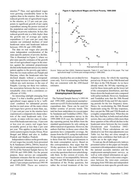
nineties. 28 Thus, real agricultural wageswere growing considerably faster in theeighties than in the nineties. But even thereduced growth rate of agricultural wagesin the nineties, at 2.5 per cent per year,points to significant growth of per capitaexpenditure among the poorer sections ofthe population and reinforces our earlierfindings on poverty reduction. In fact, thisreduced growth rate is a little higher thanthe growth rate of average per capitaexpenditure (1.5 per cent per year) thatsustains our estimated declines of ruralheadcount ratios and headcount indexesbetween 1993-94 and 1999-2000.The data on real wages also providesome independent corroboration of thestate-specific patterns of poverty decline.This is illustrated in Figure 5, where weplot state-specific estimates of the growthrate of real agricultural wages in the ninetiesagainst the estimated proportionatedecline in the headcount ratio (a very similarpattern applies to the poverty-gap index).Here the two main outliers are Punjab andHaryana, where the headcount ratio hasdeclined sharply without a correspondinglysharp increase in real wages (indeedwithout any such increase, in the case ofPunjab). Leaving out these two outliers,the association between the two series isremarkably close (with a correlation coefficientof 0.88).An interesting sidelight emerging fromFigure 5 is that a healthy growth of realagricultural wages appear to be a ‘sufficient’condition for substantial povertydecline in rural areas: all the states wherereal wages have grown at more than, say,2.5 per cent per year in the nineties haveexperienced a comparatively sharp reductionof the rural headcount ratio. Conversely,in states with low rates of reductionof the headcount ratio (say, 15 per centor less over six years), real wages haveinvariably grown at less than 2 per centper year. This applies in particular to theentire eastern region (Assam, Orissa, WestBengal and Bihar) and also to AndhraPradesh and Madhya Pradesh.Independent evidence on the growth ratesof real wages has recently been presentedby K Sundaram (2001a, 2001b), based onthe ‘employment-unemployment surveys’(EUS) of the National Sample Survey for1993-94 and 1999-2000. For the presentpurpose, these surveys are comparable.Sundaram estimates that the real earningsof agricultural labourers have grown atabout 2.5 per cent per year between 1993-94and 1999-2000. These are tentativeRural headcount ratio (adjusted)50403020100Figure 4: Agricultural Wages and Rural Poverty, 1999-2000ORKA0 2 3 4 5 6 7 8Real agricultural wageSource: Drèze and Sen (2002), Statistical Appendix, Table A 3, and Table 2a of this paper. The “realagricultural wage” is a three-year average ending in 1999-2000.estimates, based as they are on data for twoyears only. Yet it is reassuring to find thatthey are consistent with the AWI-basedestimates.II.3 The ‘Employment-Unemployment Surveys’The National Sample Survey’s 1993-94and 1999-2000 employment-unemploymentsurveys (EUS) also include consumerexpenditure data. These can be used forfurther scrutiny of poverty trends. Thistask has been undertaken in a recent paperby Sundaram and Tendulkar (2002). Theynote that the consumption survey in the1999-2000 EUS uses the traditional 30-day reporting period, but differs from thestandard questionnaire by only asking anabbreviated set of questions. However, theauthors find that, in those cases where thequestions have comparable coverage, themeans from the EUS, using the traditional30-day reporting period, are typically closeto those from the 30-day questionnaire inthe main consumption survey. Based onthis correspondence, they argue that the30-day questions in the main 1999-2000survey were not much distorted by theseven-day questions that were asked alongsidethem. In this version of events, themajor source of incomparability betweenthe 55th and 50th Rounds is not the contaminationof the 30-day questions, butrather the revised treatment of the lowBIMPUPASAPMAINDIATNWBGURAPUHAKEfrequency items, for which the reportingperiod was 30 days in the 50th Round and365 days in the 55th Round. As we havealready noted, the 365-day reporting periodfor these items pulls up the lower tailof the consumption distribution, and thusbiases down the headcount ratio comparedwith earlier methods. However, Sundaramand Tendulkar note that the 50th Roundcontained both 30-day and 365-day reportingperiods for the low frequency items.Hence, by recalculating the 50th Roundheadcounts using the 365-day responses,they can put the 50th and 55th Rounds ona roughly comparable basis. When they dothis, they find that, in both rural and urbansectors, they can confirm a little more thanthree-quarters of the official decline in theheadcount ratios between the two rounds[Sundaram and Tendulkar 2002:Table III.8]. These calculations are notidentical to our first-step adjustments (seeTable 1a), but they are close enough toinspire some confidence that both sets ofresults are in the right range.To sum up, the all-India poverty indexespresented earlier in this paper are broadlyconsistent with independent evidence fromthe national accounts statistics and theemployment-unemployment surveys, aswell as with related information on agriculturalwages. There is also some congruencebetween the inter-state contrastsemerging from NSS data and independentinformation on state-specific growth rates3738Economic and Political Weekly September 7, 2002
Proportionate decline in rural HCR806040200Source: See Figure 4.Figure 5: Wage Growth and Poverty Decline, 1993-94 to 1999-2000PU–4 –2 0 2 4 6 8 10Growth rate of real agricultural wageof ‘state domestic product’ and real agriculturalwages. The combined evidencefrom these different sources is fairly strong,even though each individual source hassignificant limitations.IIIEconomic Inequality in theNinetiesIII.1 Growth, Povertyand InequalityMABIMPWBAPORASIt is possible to think about povertydecline, as captured by standard povertyindexes, in terms of two distinct components:a growth component and a distributioncomponent. The growth componentreflects the increase of average percapita expenditure. The distribution componentcaptures any change that may takeplace in the distribution of per capita expenditureover households.This decomposition exercise is pursuedin Table 4, with reference to the headcountratio (very similar results apply to thepoverty-gap index). The first column repeatsthe headcount ratio for 1993-94from Table 2. The second column (labelled‘derivative with respect to growth’) showsour estimate of the percentage-point reductionin HCR associated with a distribution-neutral,1 per cent increase in APCEin the relevant state. To illustrate, in ruralAndhra Pradesh a 1 per cent increase inAPCE in 1993-94, with no change inHAUPINDIARATNKAGUKEdistribution, would have led to a declineof 0.9 percentage points in the ruralheadcount ratio. 29 This derivative dependspositively on the fraction of people whoare at or near the poverty line, which istypically larger in the poorer states. Thefigures in column 2 vary from –1.27 inrural Assam to –0.15 in urban Jammu andKashmir. Column 3 reproduces the totalpercentage growth between 1993-94 and1999-2000 from Table 3.If we multiply the second column (thederivative with respect to growth) by thethird column (the amount of growth), weget an estimate of the amount of povertyreduction that we would expect from growthalone, in the absence of any change in theshape of the distribution. This is an approximation,because the derivative is likelyto change as the headcount ratio falls. Incolumn 4, we report a more precise calculation:an estimate of what the headcountratio would have been in 1999-2000 if thedistributions of consumption in each statewere identical to those in 1993-94, but hadbeen shifted upwards by the amount ofgrowth in real per capita expenditure thatactually took place. This can be readilycalculated by reducing the 1993-94 povertylines by the amount of growth, andre-estimating the headcount ratios fromthese adjusted lines and the 1993-94 expendituredata. These hypothetical changescan then be compared with the actualreductions in the headcount ratios, shownin the final column. The differencebetween these last two columns is thechange in the headcount ratio that is attributableto changes in the shape of theconsumption distribution.It is important to note that the last twocolumns are highly correlated. The correlationcoefficients across the states are0.97 (rural) and 0.93 (urban), so that growthalone can predict much of the cross-statepattern of reduction in HCRs. Nevertheless,the estimates are far from identical. Inparticular, the all-India calculations showthat ‘growth alone’ would have reduced thepoverty rate by more than actually happened,implying that there was an increasein inequality that offset some of the effectsof growth, or put differently, that APCEgrowth among the poor was less than theaverage. These inequality effects varysomewhat from state to state and are muchweaker in rural than in urban areas. Inurban India, increasing inequality moderatedthe decline in the headcount ratio inall states except Delhi, Maharashtra, andJammu and Kashmir. In some cases, suchas urban Kerala and Madhya Pradesh, the‘moderating effect’ is pronounced, withactual rates of reduction only a little over halfthose predicted by the growth in the mean.For the urban sector as a whole (the lastrow of the table), the actual decline in theHCR is one and a half points lower (5.9versus 7.4 per cent) than would have beenthe case had growth been equally distributedwithin each state. This estimate, whichis the population-weighted average of thecorresponding numbers for each state,calculates what would have happened ifeach household in each state had experiencedthe average growth for that state. Analternative, and equally interesting, counterfactualis what would have happened if,between 1993-94 and 1999-2000, eachhousehold in the country had experiencedthe countrywide growth rate of 10.9 percent. Such a calculation yields an all-IndiaHCR of 21.4 per cent (for rural and urbanareas combined), compared with an actualall-India HCR of 22.7 per cent based onthe 55th Round. In other words, the all-India HCR in 1999-2000 was 1.3 percentagepoints higher than it would have been(with the same growth rate of APCE) inthe absence of any increase in inequality.III.2 Aspects of Rising InequalityThree aspects of rising economic inequalityin the nineties have come up sofar in our story. First, we found strongevidence of ‘divergence’ in per capitaEconomic and Political Weekly September 7, 2002 3739
Page 5 and 6: eal terms, with updating on the bas
Page 7 and 8: Figure 2: ‘Divergence’ of Per C
Page 12 and 13: consumption across states. Second,
Page 14 and 15: 6.05.04.03.02.01.00.0Figure 7:Progr
Page 16 and 17: and Rajasthan are two states where
Page 18 and 19: the estimated rate of increase of c
Page 20: Institute for Human Development (20

Poverty and Inequality in India: a Reexamination - Princeton University

Create successful ePaper yourself

Delete template?

Save as template?