Error Correction in Vector Network Analyzers - SDR-Kits

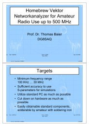
Error Correction in Vector Network AnalyzersThomas C. Baier, DG8SAQMay 19, 2009AbstractThis article describes systematic errors encountered in vector network analysis and how theycan be mathematically corrected. The focus lies on the application to a unidirectional VNA,i.e. where the 2-port device needs to be manually turned around to measure the full 2-portS-matrix.1 What does a VNA measure?Figure 1 shows a very general and abstract model of a unidirectional vector network analyzer (VNA).TXoscillatorreference signaln = a1 + b1bridge4-portreflection signalr = a1 + b1DUTport 1 port 2S 21 S 12a 1 a 2S 11 S 22 Z L u Thrub 1b 2reflection coefficient ofterminated DUT:S = b 1 /a 1Figure 1: Abstract model of a unidirectional VNA.The signal power of a TX oscillator is fed into a reflection bridge or directional coupler, which canbe described as a linear 4-port device. Port 1 is connected to the oscillator, port 2 to the DUT, port3 is the measured reflect signal r and port 4 is the measured reference signal n. Observe the waveamplitude a 1 travelling from the bridge to the DUT. This wave is partially reflected by the DUTleading to the wave amplitude b 1 .1

1.1 Measuring 1-port reflection coefficientsThe reflection coefficient S of the DUT input with its output terminated by Z L can be determinedfrom these wave amplitudes by equation 1.S = b 1a 1(1)An ideal VNA would measure a 1 as reference signal and b 1 as reflect signal and calculate the reflectioncoefficient S according to equation 1. Since the reflection bridge shown in figure 1 is a linear 4-portdevice, the signals at any port can always be described as a linear combination of the wave amplitudesa 1 and b 1 . Thus, the reflect and reference signals are of the following form:And the measurement result M is:By virtue of equation 1 we obtain the following result:r = γa 1 + δb 1 (2)n = αa 1 + βb 1 (3)M = r n = γa 1 + δb 1αa 1 + βb 1(4)M = γ + δSα + βS(5)This function is called a Moebius 1 transform. It actually contains only 3 independent parametersas one of {α,β,γ,δ} can be divided out. Thus, without loss of generality, M can be written in thefollowing way:M = S + a(6)bS + cIf the three parameters {a,b,c} are known, the input reflection coefficient S of the DUT can becalculated from the measurement result M by inverting equation 6:S = a − cMbM − 1(7)The determination of the parameters {a,b,c} is quite simple. It is just necessary to measure threecalibration standards with well known reflection coefficients, e.g. {S O ,S S ,S L }. Usually, but notnecessarily, an open a short and a load calibration standard are used. Measuring these, one obtainsthe measurement results {M O ,M S ,M L }, where by virtue of equation 6:M O = S O + abS O + cM S = S S + abS S + cM L = S L + abS L + c(8)(9)(10)1 August Ferdinand Moebius, 1790-1868, German mathematician and astronomer2

These 3 equations for the 3 unknowns {a,b,c} can easily be solved:M L (M O − M S )a =M L (M O + M S ) − 2M O M S(11)2M L − M O − M Sb =M L (M O + M S ) − 2M O M S(12)M O − M Sc =M L (M O + M S ) − 2M O M S(13)Thus, using equation 7 together with the now known parameters {a,b,c}, we can determine thereflection coefficient regardless of the details of the reflection bridge. Note, that also the outputimpedance of the reflection bridge Z S is of no importance here.How can we interpret the parameters {a,b,c}?Equation 6 can be rewritten into the formM =S + ac( b c S + 1) (14)The parameter a is closely related to what is called the directivity error [1]. If the gain of the reflectsignal or the reference signal changes, only c will change, that is why c is called a tracking error[1]. To understand the meaning of the quotient b/c is not so simple. Let’s assume that deep insideour reflection bridge there is an ideal reflection bridge with source impedance equal to the referenceimpedance Z 0 , which is usually 50Ω. This impedance is transformed to the real port impedance Z Sby an error network described by an S-parameter matrix E ij . This is shown in figure 2. The realTXoscillatormeasured signalM = b 1 /a 1idealbridgeZ 0virtualport 1errornetworkrealport 2a E 21 E 121 a 2E 11 E 22 Z Sb 1b 2DUT withreflectioncoefficient SFigure 2: Real VNA bridge built up from an ideal VNA bridge and an error network.bridge’s output impedance Z S corresponding to an output reflection coefficientS S = b ∣2 ∣∣∣a1= E 22 (15)a 2 =0Now, what would our VNA measure due to the error network if port 2 was terminated with animpedance Z with corresponding reflection coefficient S? This is calculated in the Appendix A.1.Using equation 64 and the abbreviation ∆ E = E 11 E 22 − E 12 E 21 we obtainM = Γ in = b 1= ∆ ES − E 11a 1 E 22 S − 1(16)3

Dividing enumerator and denominator by ∆ E we obtainThis is exactly of the same form as equation 6. By inspection we findNow we can calculate b/c:M = S − E 11∆ EE 22(17)∆ ES − 1∆ Ea = − E 11∆ E(18)b = E 22∆ E(19)c = − 1∆ E(20)Eb22c = ∆ E− 1∆ E= −E 22 (21)And we finally find the real port 2 reflection coefficient S S corresponding to the output impedanceof the real bridge Z S :S S = E 22 = − b c2 Measuring 2-port S-parameters2.1 Reflection measurementAs we have seen above, the bridge output impedance is of no importance when measuring 1-portreflection coefficients. This picture dramatically changes, when 2-port S-parameters are to be measuredwith the VNA depicted in figure 1. In the latter case, both impedances of the VNA, namelythe bridge output impedance Z S and the detector impedance Z L , both terminating the DUT, willinfluence the measurement result M. This is quite obvious for the reflection measurements whenlooking at equation 61 from the appendix and replacing S by S L . The input reflection coefficient ofour DUT in forward direction f is(22)S f = S 11 + S LS 12 S 211 − S 22 S L(23)If the detector impedance Z L is equal to the reference impedance Z 0 , which means S L = 0, equation23 reduces to S f = S 11 . Note, that in the general case S f depends on all four S-parameters of theDUT.If we want to measure the output reflection coefficient in backward direction b by turning the DUTaround, we have to exchange indices 1 and 2 in equation 23:S b = S 22 + S LS 21 S 121 − S 11 S L(24)4

2.2 Transmission measurementsWhen doing a transmission measurement τ, one evaluates the quotient of the detector voltage u detdivided by the reference signal n. Here we assume u det to be normalized with respect to the referenceimpedance Z 0 like the reference signal n and the reflect signal r. Thus, u det can simply be writtenin terms of wave amplitudesThus the forward transmission signal readsUsing equation 59, we can replace b 2 :The second quotient can be simplified tou det = a 2 + b 2 = b 2 S L + b 2 = b 2 (1 + S L ) (25)τ f = u detn = b 2(1 + S L )αa 1 + βb 1(26)τ f = (1 + S L)S 21 a 1·(27)1 − S 22 S L αa 1 + βb 1a 1αa 1 + βb 1=1=α + β b 1a 11α + βS f(28)Next we want to normalize τ f by a thru calibration measurement τ Thru . An ideal thru calibrationstandard yields S 11 = S 22 = 0 and S 12 = S 21 = 1. Thus for the thru calibration measurementequation 27 becomesτ Thru = (1 + S L ) ·a Tαa T + βb T= 1 + S Lα + β b TaT= 1 + S Lα + βS L(29)Note that the wave amplitudes depend on the DUT and are different in equation 29 from those inequation 27. Now we can normalize the forward transmission signal dividing it by the thru calibrationmeasurement:T f =τ fτ Thru=(1+S L )S 21 11−S 22 S L·α+βS f1+S L=α+βS LS 211 − S 22 S L· α + βS Lα + βS f=S 211 − S 22 S L· 1 + β α S L1 + β α S f(30)Note, that β/α = b/c = −S S as can be seen from equations 5, 6 and 22. Thus we findT f =S 211 − S 22 S L· 1 − S SS L1 − S S S f(31)We can find the backward thru response from this by swapping indices 1 and 2 and replacing subscriptf by b.S 12T b = · 1 − S SS L(32)1 − S 11 S L 1 − S S S bNow, we have a set of 4 measurement results S f , S b , T f and T b (equations 23, 24, 31, 32), which alldepend on all four S-parameters S 11 , S 12 , S 21 , S 22 to be determined. Note that all parameters are5

known or can be measured, namely a, b, c and S S = −b/c are known from the reflect calibration andS L can be measured with the reflect calibrated bridge during the thru calibration.It remains to solve equations 23, 24, 31 and 32 for the unknown S-parameters S 11 , S 12 , S 21 , S 22 , sothe VNA can actually calculate the S-parameters from the measurement results.2.3 Calculating the S-parameters from the measurement resultsThe following normalization steps are not straight forward but were made to bring my equations tothe same form as those published by Agilent [1]. In that course, my error terms can be compared toAgilent’s notation.First, the reflect measurements from equations 23 and 24 are rewritten. These reflection coefficientscan be transformed to the uncalibrated measurement results M F and M B by virtue of equation 6Now we perform a renormalization:M f = S f + abS f + cM b = S b + abS b + c(33)(34)M 11 = c2 M f − acc − ab= cS fbS f + c(35)M 22 = c2 M b − acc − abWe also renormalize the thru measurements T f and T b := cS bbS b + c(36)M 21 =M 12 =T f1 − S S S L(37)T b1 − S S S L(38)As can easily be seen 2 , solving these M ij for the desired S-parameters yields2 Remark of the author: after several pages of tedious calculations6

S 11 = M 11(M 22 S S + 1) − M 12 M 21 S LDS 21 = M 21(1 − M 22 (S L − S S ))D(39)(40)S 22 = M 22(M 11 S S + 1) − M 12 M 21 S LDS 12 = M 12(1 − M 11 (S L − S S ))D(41)(42)D = (S S M 11 + 1)(S S M 22 + 1) − S 2 LM 12 M 21 (43)These equations are identical with those published in Agilent’s paper [1] on page 20 if the identificationsdescribed in appendix A.2 are applied.Now, just for completeness, we can replace the M ij -terms through equations 35-38:∆ = b 2 S 2 L(S b S f T b T f − 1) + bcS L (S b S L T b T f + S f S L T b T f − 2) + c 2 (S 2 LT b T f − 1) (44)S 11 = b2 S f S L (S b T b T f − S L ) + bcS L (S b T b T f + S f (T b T f − 2)) + c 2 (S L T b T f − S f )∆S 21 = T f(bS f + c)(bS L + c)(S b S L − 1)∆S 22 = b2 S b S L (S f T b T f − S L ) + bcS L (S b (T b T f − 2) + S f T b T f ) + c 2 (S L T b T f − S b )∆S 12 = T b(bS b + c)(bS L + c)(S f S L − 1)∆(45)(46)(47)(48)7

Assuming that the detector has an ideal match, i.e. S L = 0, these equations reduce toS 11 = S f (49)S 21 = T f (1 + b c S f)= T f (1 − S S S f ) (50)= T fa · b − cc(b · M f − 1)S 22 = S b (51)S 12 = T b (1 + b c S b)= T b (1 − S S S b ) (52)= T ba · b − cc(b · M b − 1)Note that in the last four equations equations the forward and backward directions are decoupled.This might be a good alternative if only one signal direction can be measured and Z L is close to Z 0 .Generally, Z L can be controlled more easily than Z S . Also note, that these decoupled equations stillcompensate for a nonperfect bridge output impedance Z S .An even better approximation for the transmission correction is the so called ”enhanced responsecalibration” (ERC) [3]. It can be derived from equation 31 by setting S 22 = 0.S 21 = T f · 1 − S SS 111 − S S S L(53)By doing so, one suppresses multiple reflections between DUT output and detector input. This is agood approximation for reasonably well matched DUTs. For highly mismatched DUTs this can stillbe a good approximation, if the detector reflection coefficient S L is close to zero as was shown in theprevious approximation.2.4 Isolation calibrationSo far, we have only made use of 5 independent parameters in our calibration scheme, namely a, b, c,S L and τ Thru in forward direction. The same 5 parameters are recycled for the backward direction.So, we have used a total of calibration 10 parameters so far, which means 2 parameters are missing toa 12-term error correction. The two missing parameters are the instrument isolation in forward andbackward direction. For the unidirectional VNA both are identical. As can be seen from Agilent’sequations 74 and 76, the isolation measurement is simply subtracted from the thru measurement.This is only an approximation. It does not take into account that the isolation may depend on theterminations of the TX and RX ports. Still, it is useful if either the isolation is very good or if the8

dependencies on TX and RX port terminations are weak.AAppendixA.1 Relationship between input reflection coefficient and output terminationof a 2-porta 1port 1 port 2S 21 S 12 a 2S 11 S 22b 1b 2two port deviceaS b22Z ZZ Z00Figure 3: Two-port device terminated with impedance Z.The following relationship hold between the wave amplitudes shown in figure 3:( ) ( ) ( )b1 S11 S= 12 a1·b 2 S 21 S 22 a 2(54)This can also be written as two scalar equations:b 1 = S 11 a 1 + S 12 a 2 (55)b 2 = S 21 a 1 + S 22 a 2 (56)Since the wave b 2 is reflected by the termination impedance Z with corresponding reflection coefficientS, we can write:S = a 2b 2(57)or by virtue of equation 56Solving for b 2 we obtainb 2 = S 21 a 1 + S 22 Sb 2 (58)b 2 = S 21a 11 − SS 22(59)Now we can calculate the input reflection coefficient for port 1 from equation 55:Γ in = b 1a 1= S 11 + S 12a 2a 1(60)Inserting b 2 from 56 leads toΓ in = S 11 + SS 12S 211 − S 22 S9(61)

Bringing this to a common denominatorΓ in = (S 11S 22 − S 12 S 21 )S − S 11S 22 S − 1(62)and using an abbreviation for the determinant of the S-matrix∆ S = S 11 S 22 − S 12 S 21 (63)we obtain the final resultΓ in = b 1= ∆ SS − S 11a 1 S 22 S − 1(64)A.2 Identifications of Agilent’s error termsThe error terms in [1] can be identified with ours.A.2.1Forward error termse 11 = S S = − b c(65)e 22 = S L (66)e 00 = a c(67)e 10 e 01 = 1 c − abc 2 (68)Note that e 10 e 32 is related to the thru calibration. It is effectively removed in our equations byworking with the renormalized M ij ’s , see section A.2.3.A.2.2Backward error termse ′ 11 = S L (69)e ′ 22 = S S = − b c(70)e ′ 33 = a c(71)e ′ 23e ′ 32 = 1 c − abc 2 (72)Note that e ′ 23e ′ 01 is related to the thru calibration. It is effectively removed in our equations byworking with the renormalized M ij ’s , see section A.2.3.10

A.2.3 M ij -TermsS 11M − e 00e 10 e 01= M 11 = c2 M f − acc − ab= cS fbS f + c(73)S 21M − e 30e 10 e 32= M 21 =T f1 − S S S L(74)S 22M − e ′ 33e ′ 23e ′ 32= M 22 = c2 M b − acc − ab= cS bbS b + c(75)S 12M − e ′ 03e ′ 23e ′ 01= M 12 =T b1 − S S S L(76)11

A.3 Comparison of notationsThe following translation table is useful when comparing literature results from various sources.HP notation [2] vs. Agilent notation [1] vs. my notationForward direction:Backward direction:E DF = e 00 = a c(77)E SF = e 11 = S S (78)E RF = e 10 e 01 = 1 c − abc 2 (79)E LF = e 22 = S L (80)E TF = e 10 e 32 = τ Thru · (1 − S S S L ) (thru cal measurement) (81)E XF = e 30 (isolation) (82)S 21M = S 21M = τ f (83)S 11M = S 11M = M f (84)E DR = e ′ 33 = a c(86)E SR = e ′ 22 = S S (87)E RR = e ′ 23e ′ 32 = 1 c − abc 2 (88)E LR = e ′ 11 = S L (89)(85)E TR = e ′ 23e ′ 01 = τ Thru · (1 − S S S L ) (thru cal measurement) (90)E XR = e ′ 03 (isolation) (91)S 12M = S 12M = τ b (92)S 22M = S 22M = M b (93)(94)12

References[1] Doug Rytting, ”Network Analyzer Error Models and Calibration Methods”, Agilent.The pdf document can be downloaded from:http://cpd.ogi.edu/IEEE-MTT-ED/Network%20Analyzer%20Error%20Models%20and%20Calibration%20Methods.pdf[2] User’s Guide, HP 8753D Network Analyzer, Hewlett-Packard.The pdf document can be downloaded from:http://cp.literature.agilent.com/litweb/pdf/08753-90257.pdf[3] Agilent application note AN 1287-3: ”Applying Error Correction to Network Analyzer Measurements”The pdf document can be downloaded from:http://cp.literature.agilent.com/litweb/pdf/5965-7709E.pdfBAcknowledgementsMany thanks to Paul Kiciak N2PK, who brought up this subject to me and who showed me thatthe 12-term correction scheme is also feasible to unidirectional VNAs. He has brought the enhancedresponse calibration to my notice. He has also provided me with lots of literature and was alwayswilling to discuss my results. Last but not least he revued this document and helped to get the bugsout.13