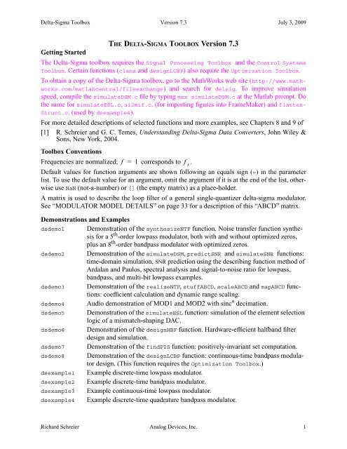
THE DELTA-SIGMA TOOLBOX Version 7.3

Delta-Sigma Toolbox Version 7.3 July 3, 2009OTHER SELECTED FUNCTIONSDelta-Sigma Utilitymod1, mod2Set the ABCD matrix, NTF and STF of the standard 1 st and 2 nd -order modulators.snr = calculateSNR(hwfft,f)Estimate the SNR given the in-band bins of a Hann-windowed FFT and the location ofthe input signal.[A B C D] = partitionABCD(ABCD, m)Partition ABCD into A, B, C, D for an m-input state-space system.H_inf = infnorm(H)Compute the infinity norm (maximum absolute value) of a z-domain transfer function.See evalTF.y = impL1(ntf,n=10)Compute n points of the impulse response from the comparator output back to thecomparator input for the given NTF.y = pulse(S,tp=[0 1],dt=1,tfinal=10,nosum=0)Compute the sampled pulse response of a continuous-time system.sigma_H = rmsGain(H,f1,f2)Compute the root mean-square gain of the discrete-time transfer function H in thefrequency band (f1,f2).General Utilitydbv(), dbp(), undbv(), undbp(), dbm(), undbm()The dB equivalent of voltage/power quantities, and their inverse functions.window = ds_hann(N)A Hann window of length N. Unlike MATLAB’s original hanning function, ds_hanndoes not smear tones which are located exactly in an FFT bin (i.e. tones having anintegral number of cycles in the given block of data). MATLAB 6’s hanning(N,’periodic’)function and MATLAB 7’s hann(N,’periodic’) function dothe same as ds_hann(N).GraphingplotPZ(H,color='b',markersize=5,list=0)Plot the poles and zeros of a transfer function.plotSpectrum(X,fin,fmt)Plot a smoothed spectrumfigureMagic(xRange,dx,xLab, yRange,dy,yLab, size)Performs a number of formatting operations for the current figure, including axislimits, ticks and labelling.printmif(file,size,font,fig)Print a figure to an Adobe Illustrator file and then use ai2mif to convert it toFrameMaker MIF format. ai2mif is an improved version of the function of the samename originally written by Deron Jackson .[f,p] = logsmooth(X,inBin,nbin)Smooth the FFT X, and convert it to dB. See also bplogsmooth and bilogplot.Richard Schreier Analog Devices, Inc. 4

Delta-Sigma Toolbox Version 7.3 July 3, 2009synthesizeChebyshevNTFSynopsis: ntf = synthesizeChebyshevNTF(order=3,OSR=64,opt=0,H_inf=1.5,f0=0)Synthesize a noise transfer function (NTF) for a delta-sigma modulator. synthesizeNTF assumesthat magnitude of the denominator of the NTF is approximately constant in the passband. Whenthe OSR or H_inf are low, this assumption breaks down and synthesizeNTF yields a non-optimalNTF. synthesizeChebyshevNTF creates non-optimal NTFs, but fares better than synthesizeNTFin the aforementioned circumstances.Arguments and OutputSame as synthesizeNTF, except that the f0 argument is not supported yet.ExamplesCompare the NTFs created by synthesizeNTF and synthesizeChebyshevNTF when OSR is low:>> OSR = 4; order = 8; H_inf = 3;>> H1 = synthesizeNTF(order,OSR,1,H_inf);>> H3 = synthesizeChebyshevNTF(order,OSR,1,H_inf);Pole-Zero PlotMagnitude Response10–20rms gain -12 dBrms gain -24 dB0–1–1 0 1–40synthesizeNTF–60synthesizeChebyshevNTF–800 0.1 0.2 0.3 0.4 0.5Repeat for H_inf low:>> OSR = 32; order = 5; H_inf = 1.2;>> H1 = synthesizeNTF(order,OSR,1,H_inf);>> H3 = synthesizeChebyshevNTF(order,OSR,1,H_inf);Pole-Zero PlotMagnitude Response100–20–40rms gain -33 dBrms gain -38 dB–1–1 0 1synthesizeNTF–60synthesizeChebyshevNTF–800 0.1 0.2 0.3 0.4 0.5Richard Schreier Analog Devices, Inc. 7

Delta-Sigma Toolbox Version 7.3 July 3, 2009simulateDSMSynopsis: [v,xn,xmax,y] = simulateDSM(u,ABCD|ntf,nlev=2,x0=0)Simulate a delta-sigma modulator with a given input. For maximum speed, make sure that thecompiled mex file is on your search path (by typing which simulateDSM at the MATLAB prompt).Argumentsu The input sequence to the modulator, given as a m×N row vector. m is the numberof inputs (usually 1). Full-scale corresponds to an input of magnitude nlev−1.ABCD A state-space description of the modulator loop filter.ntfThe modulator NTF, given in zero-pole form.The modulator STF is assumed to be unity.nlevThe number of levels in the quantizer. Multiple quantizers are indicated by makingnlev an array.x0The initial state of the modulator.OutputvxnxmaxyThe samples of the output of the modulator, one for each input sample.The internal states of the modulator, one for each input sample, given as ann × N matrix.The maximum absolute values of each state variable.The samples of the quantizer input, one per input sample.ExampleSimulate a 5 th -order binary modulator with a half-scale sine-wave input and plot its output in thetime and frequency domains.>> OSR = 32; H = synthesizeNTF(5,OSR,1);>> N = 8192; fB = ceil(N/(2*OSR));>> f=85; u = 0.5*sin(2*pi*f/N*[0:N-1]);>> v = simulateDSM(u,H);u, vdBFS/NBW+10-10 10 20 30 40 50 60 70 80sample number0-40-80SNR = 82.5dBNBW=0.00018-1200 0.1 0.2 0.3 0.4 0.5normalized frequency (1 → f s )t = 0:85;stairs(t, u(t+1),'g');hold on;stairs(t,v(t+1),'b');axis([0 85 -1.2 1.2]);ylabel('u, v');spec=fft(v.*ds_hann(N))/(N/4);plot(linspace(0,0.5,N/2+1), ...dbv(spec(1:N/2+1)));axis([0 0.5 -120 0]);grid on;ylabel('dBFS/NBW')snr=calculateSNR(spec(1:fB),f);s=sprintf('SNR = %4.1fdB\n',snr)text(0.25,-90,s);s=sprintf('NBW=%7.5f',1.5/N);text(0.25, -110, s);Richard Schreier Analog Devices, Inc. 8

Delta-Sigma Toolbox Version 7.3 July 3, 2009simulateSNRSynopsis: [snr,amp] = simulateSNR(ntf|ABCD|function,OSR,amp,f0=0,nlev=2,f=1/(4*OSR),k=13,quadrature=0)Simulate a delta-sigma modulator with sine wave inputs of various amplitudes and calculate thesignal-to-noise ratio (SNR) in dB for each input.ArgumentsntfThe modulator NTF, given in zero-pole form.ABCD A state-space description of the modulator loop filter.function The name of a function taking the input signal as its sole argument.OSR The oversampling ratio. OSR is used to define the “band of interest.”amp A row vector listing the amplitudes to use. Defaults to [-120 -110...-20 -15 -10 -9-8 … 0] dB, where 0 dB means a full-scale (peak value = nlev-1) sine wave.f0The center frequency of the modulator. f0≠0 corresponds to a bandpass modulator.nlevThe number of levels in the quantizer.fThe normalized frequency of the test sinusoid; a check is made that the test frequencyis in the band of interest. The frequency is adjusted so that it lies preciselyin an FFT bin.k The number of time points used for the FFT is 2 k .quadrature A flag indicating that the system being simulated is quadrature. This flag is setautomatically if either ntf or ABCD are complex.OutputsnrampA row vector containing the SNR values calculated from the simulations.A row vector listing the amplitudes used.ExampleCompare the SNR vs. input amplitude curve for a fifth-order modulator determined by the describingfunction method with that determined by simulation.>> OSR = 32; H = synthesizeNTF(5,OSR,1);>> [snr_pred,amp] = predictSNR(H,OSR);>> [snr,amp] = simulateSNR(H,OSR);SNR dB1009080706050403020peak SNR = 84.9dB100-100 -80 -60 -40 -20 0Input Level, dBplot(amp,snr_pred,'b',amp,snr,'gs');grid on;figureMagic([-100 0], 10, 2, ...[0 100], 10, 1);xlabel('Input Level, dB');ylabel('SNR dB');s=sprintf('peak SNR = %4.1fdB\n',...max(snr));text(-65,15,s);Richard Schreier Analog Devices, Inc. 9

Delta-Sigma Toolbox Version 7.3 July 3, 2009realizeNTFSynopsis: [a,g,b,c] = realizeNTF(ntf,form='CRFB',stf=1)Convert a noise transfer function (NTF) into a set of coefficients for a particular modulator topology.ArgumentsntfformstfThe modulator NTF, given in zero-pole form (i.e. a zpk object).A string specifying the modulator topology.CRFB Cascade-of-resonators, feedback form.CRFF Cascade-of-resonators, feedforward form.CIFB Cascade-of-integrators, feedback form.CIFF Cascade-of-integrators, feedforward form.… D Any of the above, but the quantizer is delaying.Structures are described in detail in “MODULATOR MODEL DETAILS” onpage 33.The modulator STF, specified as a zpk object. Note that the poles of the STF mustmatch those of the NTF in order to guarantee that the STF can be realized withoutthe addition of extra state variables.Outputa Feedback/feedforward coefficients from/to the quantizer ( 1 × n).g Resonator coefficients ( 1 × n ⁄ 2 ).b Feed-in coefficients from the modulator input to each integrator ( 1 × n + 1).c Integrator inter-stage coefficients. ( 1 × n. In unscaled modulators, c is all ones.)ExampleDetermine the coefficients for a 5 th -order modulator with the cascade-of-resonators structure,feedback (CRFB) form.>> H = synthesizeNTF(5,32,1);>> [a,g,b,c] = realizeNTF(H,'CRFB')a = 0.0007 0.0084 0.0550 0.2443 0.5579g = 0.0028 0.0079b = 0.0007 0.0084 0.0550 0.2443 0.5579 1.0000c = 1 1 1 1 1See AlsorealizeNTF_ct on page 14 to realize an NTF with a continuous-time loop filter.Richard Schreier Analog Devices, Inc. 10

Delta-Sigma Toolbox Version 7.3 July 3, 2009stuffABCDSynopsis: ABCD = stuffABCD(a,g,b,c,form='CRFB')Calculate the ABCD matrix given the parameters of a specified modulator topology.ArgumentsagbcformOutputABCDFeedback/feedforward coefficients from/to the quantizer. 1 × nResonator coefficients. 1 × n ⁄ 2Feed-in coefficients from the modulator input to each integrator.Integrator inter-stage coefficients. 1 × nsee realizeNTF on page 10 for a list of supported structures.A state-space description of the modulator loop filter.1 × n + 1mapABCD[a,g,b,c] = mapABCD(ABCD,form='CRFB')Calculate the parameters for a specified modulator topology, assuming ABCD fits that topology.ArgumentsABCDformOutputagbcA state-space description of the modulator loop filter.see realizeNTF on page 10 for a list of supported structures.Feedback/feedforward coefficients from/to the quantizer. 1 × nResonator coefficients. 1 × n ⁄ 2Feed-in coefficients from the modulator input to each integrator.Integrator inter-stage coefficients. 1 × n1 × n + 1Richard Schreier Analog Devices, Inc. 11

Delta-Sigma Toolbox Version 7.3 July 3, 2009scaleABCDSynopsis: [ABCDs,umax]=scaleABCD(ABCD,nlev=2,f=0,xlim=1,ymax=nlev+5,umax,N=1e5)Scale the ABCD matrix so that the state maxima are less than a specified limit. The maximum stableinput is determined as a side-effect of this process.ArgumentsABCDnlevfxlimymaxOutputABCDsumaxA state-space description of the modulator loop filter.The number of levels in the quantizer.The normalized frequency of the test sinusoid.The limit on the states. May be given as a vector.The threshold for judging modulator stability. If the quantizer input exceedsymax, the modulator is considered to be unstable.The scaled state-space description of the modulator loop filter.The maximum stable input. Input sinusoids with amplitudes below this valueshould not cause the modulator states to exceed their specified limits.Richard Schreier Analog Devices, Inc. 12

Delta-Sigma Toolbox Version 7.3 July 3, 2009calculateTFSynopsis: [ntf,stf] = calculateTF(ABCD,k=1)Calculate the NTF and STF of a delta-sigma modulator.ArgumentsABCDkOutputntfstfA state-space description of the modulator loop filter.The value to use for the quantizer gain.The modulator NTF, given as an LTI system in zero-pole form.The modulator STF, given as an LTI system in zero-pole form.ExampleRealize a fifth-order modulator with the cascade-of-resonators structure, feedback form. Calculatethe ABCD matrix of the loop filter and verify that the NTF and STF are correct.>> H = synthesizeNTF(5,32,1)Zero/pole/gain:(z-1) (z^2 - 1.997z + 1) (z^2 - 1.992z + 1)----------------------------------------------------------(z-0.7778) (z^2 - 1.613z + 0.6649) (z^2 - 1.796z + 0.8549)Sampling time: 1>> [a,g,b,c] = realizeNTF(H)a =0.0007 0.0084 0.0550 0.2443 0.5579g =0.0028 0.0079b =0.0007 0.0084 0.0550 0.2443 0.5579 1.0000c =1 1 1 1 1>> ABCD = stuffABCD(a,g,b,c)ABCD =1.0000 0 0 0 0 0.0007 -0.00071.0000 1.0000 -0.0028 0 0 0.0084 -0.00841.0000 1.0000 0.9972 0 0 0.0633 -0.06330 0 1.0000 1.0000 -0.0079 0.2443 -0.24430 0 1.0000 1.0000 0.9921 0.8023 -0.80230 0 0 0 1.0000 1.0000 0>> [ntf,stf] = calculateTF(ABCD)Zero/pole/gain:(z-1) (z^2 - 1.997z + 1) (z^2 - 1.992z + 1)----------------------------------------------------------(z-0.7778) (z^2 - 1.613z + 0.6649) (z^2 - 1.796z + 0.8549)Sampling time: 1Zero/pole/gain:1Static gain.Richard Schreier Analog Devices, Inc. 13

Delta-Sigma Toolbox Version 7.3 July 3, 2009realizeNTF_ctSynopsis: [ABCDc,tdac2] = realizeNTF_ct( ntf, form='FB', tdac, ordering=[1:n],bp=zeros(…), ABCDc)Realize a noise transfer function (NTF) with a continuous-time loop filter.ArgumentsntfformtdacorderingbpABCDcOutputABCDctdac2The modulator NTF, specified as an LTI object in zero-pole form.A string specifying the modulator topology.FB Feedback form.FF Feedforward form.The timing for the feedback DAC(s). If tdac(1)≥1, direct feedback terms areadded to the quantizer. Multiple timings (one or more per integrator) for the FBtopology can be specified by making tdac a cell array, e.g.tdac = {[1,2]; [1 2]; {[0.5 1],[1 1.5]}; []};In this example, the first two integrators have DACs with [1,2] timing, the thirdhas a pair of dacs, one with [0.5 1] timing and the other with [1 1.5] timing,and there is no direct feedback DAC to the quantizer.A vector specifying which NTF zero-pair to use in each resonator. Default is forthe zero-pairs to be used in the order specified in the NTF.A vector specifying which resonator sections are bandpass. The default(zeros(...)) is for all sections to be lowpass.The loop filter structure, in state-space form. If this argument is omitted, ABCDcis constructed according to form.A state-space description of the CT loop filterA matrix with the DAC timings, including ones that were automatically added.ExampleRealize the NTF ( 1 – z 1 ) 2 with a CT system (cf. the example on page 15).>> ntf = zpk([1 1],[0 0],1,1);>> [ABCDc,tdac2] = realizeNTF_ct(ntf,'FB')ABCDc =0 0 1.0000 -1.00001.0000 0 0 -1.50000 1.0000 0 0.0000tdac2 =-1 -10 1Richard Schreier Analog Devices, Inc. 14

Delta-Sigma Toolbox Version 7.3 July 3, 2009mapCtoDSynopsis: [sys, Gp] = mapCtoD(sys_c,t=[0 1],f0=0)Map a MIMO continuous-time system to a SIMO discrete-time equivalent. The criterion forequivalence is that the sampled pulse response of the CT system must be identical to the impulseresponse of the DT system. I.e. if y c is the output of the CT system with an input v c taken from aset of DACs fed with a single DT input v, then y, the output of the equivalent DT system withinput v satisfies y() n = y c( n - ) for integer n. The DACs are characterized by rectangular impulseresponses with edge times specified in the t matrix.Argumentssys_ctf0OutputsysGpThe LTI description of the CT system.The edge times of the DAC pulse used to make CT waveforms from DT inputs.Each row corresponds to one of the system inputs; [-1 -1] denotes a CT input.The default is [0 1] for all inputs except the first, which is assumed to be a CTinput.The (normalized) frequency at which the Gp filters' gains are to be set to unity.Default 0 (DC).The LTI description for the DT equivalent.The mixed CT/DT prefilters which form the samples fed to each state for the CTinputs.Reference[1] R. Schreier and B. Zhang, “Delta-sigma modulators employing continuous-time circuitry,”IEEE Transactions on Circuits and Systems I, vol. 43, no. 4, pp. 324-332, April 1996.ExampleMap the standard second-order CT modulator shown below to its DT equivalent and verify thatthe NTF. is ( 1 – z – 1 ) 2 x˙x˙u cQ v∫ ∫1c0 0 1 – 1 1c(clocked)x˙x˙=2c1 0 0 – 1.5 2c–1–1.5 v u ccDACy c 0 1 0 0>> LFc = ss([0 0;1 0], [1 -1;0 -1.5], [0 1], [0 0]);>> tdac = [0 1];>> [LF,Gp] = mapCtoD(LFc,tdac);>> ABCD = [LF.a LF.b; LF.c LF.d];>> H = calculateTF(ABCD)Zero/pole/gain:(z-1)^2-------z^2Sampling time: 1v cRichard Schreier Analog Devices, Inc. 15

Delta-Sigma Toolbox Version 7.3 July 3, 2009evalTFPSynopsis: H = evalTFP(Hs,Hz,f)Use this function to evaluate the signal transfer function of a continuous-time (CT) system. In thiscontext Hs is the open-loop response of the loop filter from the u input and Hz is the closed-loopnoise transfer function.ArgumentsHsHzfA continuous-time transfer function in zpk form.A discrete-time transfer function in zpk form.A vector of frequencies.OutputH The value of H s( j2πf )H z( e j2πf ).evalTFP attempts to cancel poles in with zeros in .See AlsoevalMixedTF is a more advanced version of this function which is used to evaluate the individualfeed-in transfer functions of a CT modulator.ExamplePlot the STF of the 2 nd -order CT system depicted on page 15.Ac = [ 0 0; 1 0]; Bc = [1 -1; 0 -1.5];Cc = [0 1]; Dc = [0 0];LFc = ss(Ac, Bc, Cc, Dc);L0c = zpk(ss(Ac,Bc(:,1),Cc,Dc(1)));tdac = [0 1];[LF,Gp] = mapCtoD(LFc,tdac);ABCD = [LF.a LF.b; LF.c LF.d];H = calculateTF(ABCD);% Yields H=(1-z^-1)^2f = linspace(0,2,300);STF = evalTFP(L0c,H,f);plot(f,dbv(STF));0H sH z|STF| (dB)–20–40–600 0.5 1 1.5 2frequencyRichard Schreier Analog Devices, Inc. 16

Delta-Sigma Toolbox Version 7.3 July 3, 2009simulateESLSynopsis: [sv,sx,sigma_se,max_sx,max_sy]= simulateESL(v,mtf,M=16,dw=[1…], sx0=[0…])Simulate the element selection logic (ESL) of a multi-element DAC using a particular mismatchshapingtransfer function (mtf).[1] R. Schreier and B. Zhang “Noise-shaped multibit D/A convertor employing unit elements,”Electronics Letters, vol. 31, no. 20, pp. 1712-1713, Sept. 28 1995.ArgumentsvA vector containing the number of elements to enable. Note that the output ofsimulateDSM must be offset and scaled in order to be used here as v must be inMthe range [ 0,∑ dw()i ] .imtfThe mismatch-shaping transfer function, given in zero-pole form.MThe number of elements.dwA vector containing the weight associated with each element.sx0 An n × M matrix containing the initial state of the element selection logic.OutputsvThe selection vector: a vector of zeros and ones indicating which elements toenable.sx An n × M matrix containing the final state of the element selection logic.sigma_se The rms value of the selection error, se = sv – sy. sigma_se may be used toanalytically estimate the power of in-band noise caused by element mismatch.max_sx The maximum value attained by any state in the ESL.max_sy The maximum value attained by any component of the (un-normalized) “desiredusage” vector.vsusyvectorquantizer-min()MTF -1seMsvBlock diagram of the Element Selection LogicRichard Schreier Analog Devices, Inc. 17

Delta-Sigma Toolbox Version 7.3 July 3, 2009Example (From dsdemo5)Compare the usage patterns and example spectra for a 16-element DAC driven with thermometercoded,1 st -order mismatch-shaped and 2 nd -order mismatch-shaped data generated by a 3 rd -ordermulti-bit modulator.>> ntf = synthesizeNTF(3,[],[],4);>> M = 16;>> N = 2^14;>> fin = round(0.33*N/(2*12));>> u = M/sqrt(2)*sin((2*pi/N)*fin*[0:N-1]);>> v = simulateDSM(u,ntf,M+1);>> v = (v+M)/2; % scale v to [0,M]>> sv0 = thermometer(v,M);>> mtf1 = zpk(1,0,1,1); %First-order shaping>> sv1 = simulateESL(v,mtf1,M);>> mtf2 = zpk([ 1 1 ], [ 0 0 ], 1, 1); %Second-order shaping>> sv2 = simulateESL(v,mtf2,M);>> ue = 1 + 0.01*randn(M,1); % 1% mismatch>> dv0 = ue' * sv0;>> spec0 = fft(dv0.*ds_hann(N))/(M*N/8);>> plotSpectrum(spec0,fin,'g');…Thermometer-CodingElements1% mismatch00 10 20First-Order Shaping0 10 20Second-Order ShapingPSD (dBFS/NBW)–50–100–150Thermometer1 st –Order2 ndt –OrderNo MismatchNBW=9×10 –5–20010 –3 10 –2 frequency10 –10 10 20TimeRichard Schreier Analog Devices, Inc. 18

Delta-Sigma Toolbox Version 7.3 July 3, 2009synthesizeQNTFSynopsis: ntf = synthesizeQNTF(order=3,OSR=64,f0=0,NG=-60,ING=-20,n_im=order/3)Synthesize a noise transfer function (NTF) for a quadrature delta-sigma modulator.ArgumentsorderOSRf0NGINGn_imOutputntfThe order of the NTF.The oversampling ratio.The center frequency of the modulator. f0≠0 yields a bandpass modulator;f0=0.25 puts the center frequency at f s⁄ 4.The rms in-band noise gain (dB).The rms image-band noise gain (dB).Number of image-band zeros.The modulator NTF, given as an LTI object in zero-pole form.BugsALPHA VERSION. This function uses an experimental ad hoc method that is neither optimal norrobust.Example (From dsexample4)Fourth-order, OSR = 32 , f 0= 1 ⁄ 16 bandpass NTF with an rms in-band noise gain of –50 dBand an image-band noise gain of –10 dB.>> ntf = synthesizeQNTF(4,32,1/16,-50,-10);Zero/pole/gain:(z-(0.953+0.3028i)) (z^2 - 1.848z + 1) (z-(0.888+0.4598i))--------------------------------------------------------------------------------------(z-(0.8088+0.002797i)) (z-(0.5913+0.2449i)) (z-(0.6731-0.2788i)) (z-(0.5739+0.5699i))Sampling time: 1Frequency ResponsePoles and Zeros10–20–10dBInf-norm of H=1.792-norm of H=1.540–40–50dB–60–1–1 0 1–80–0.5 –0.375 –0.25 –0.125 0 0.125 0.25 0.375 0.5frequencyRichard Schreier Analog Devices, Inc. 19

Delta-Sigma Toolbox Version 7.3 July 3, 2009simulateQDSMSynopsis: [v,xn,xmax,y] = simulateQDSM(u,ABCD|ntf,nlev=2,x0=0)Simulate a quadrature delta-sigma modulator with a given input. For improved simulation speed,use simulateDSM with a 2-input/2-output ABCDr argument as indicated in the example below.Argumentsu The input sequence to the modulator, given as a 1 × N row vector.Full-scale corresponds to an input of magnitude nlev−1.ABCD A state-space description of the modulator loop filter.ntfThe modulator NTF, given in zero-pole form.The modulator STF is assumed to be unity.nlevThe number of levels in the quantizer. Multiple quantizers are indicated by makingnlev an array.x0The initial state of the modulator.OutputvxnxmaxyThe samples of the output of the modulator, one for each input sample.The internal states of the modulator, one for each input sample, given as ann × N matrix.The maximum absolute values of each state variable.The samples of the quantizer input, one per input sample.ExampleSimulate a 4 th -order 9-level f 0= 1 ⁄ 16 quadrature modulator with a half-scale sine-wave inputand plot its output in the time and frequency domains.nlev = 9; f0 = 1/16; osr = 32; M = nlev-1;ntf = synthesizeQNTF(4,osr,f0,-50,-10);ABCD = realizeQNTF(ntf,'FF');N = 64*osr; f = round((f0+0.3*0.5/osr)*N)/N; ABCDr = mapQtoR(ABCD);u = 0.5*M*exp(2i*pi*f*[0:N-1]);ur = [real(u); imag(u)];v = simulateQDSM(u,ntf,nlev);vr=simulateDSM(ur,ABCDr,nlev*[1;1]);faster code v = vr(1,:) + 1i*vr(2,:);realimagt = 0:25;subplot(211)plot(t, real(u(t+1)),'g');hold on;stairs(t,real(v(t+1)),'b');figureMagic(…)ylabel('real');840–4–80 10 20840–4–80 10 20spec = fft(v.*ds_hann(N))/(M*N/2);spec = [fftshift(spec) spec(N/2+1)];plot(linspace(-0.5,0.5,N+1), dbv(spec))figureMagic([-0.5 0.5],1/16,2, [-120 0],10,2)ylabel('dBFS/NBW')[f1 f2] = ds_f1f2(osr,f0,1);fb1 = round(f1*N); fb2 = round(f2*N);fb = round(f*N)-fb1;snr = calculateSNR(spec(N/2+1+[fb1:fb2]),fb);text(f,-10,sprintf(' SNR = %4.1fdB\n',snr));text(0.25, -105, sprintf('NBW=%0.1e',1.5/N));dBFS/NBW0–20–40–60–80SNR = 78.3dB–100NBW= 7.3×10 –4–120–0.5 –0.375 –0.25 –0.125 0 0.125 0.25 0.375 0.5Richard Schreier Analog Devices, Inc. 20

Delta-Sigma Toolbox Version 7.3 July 3, 2009realizeQNTFSynopsis: ABCD = realizeQNTF(ntf,form='FB',rot=0,bn)Convert a quadrature noise transfer function (NTF) into an ABCD matrix for the desired structure.ArgumentsntfformrotbnThe modulator NTF, given in zero-pole form (i.e. a zpk object).A string specifying the modulator topology.FB FeedbackPFB Parallel feedbackFF FeedforwardPFF Parallel feedforwardFBD FB with delaying quantizer. NOT SUPPORTED YETFFD FF with delaying quantizer. NOT SUPPORTED YETrot =1 means rotate states to make as many coefficients as possible realThe coefficient of the auxiliary DAC for form = ’FF’OutputABCD State-space description of the loop filter.Example (From dsexample4)Determine coefficients for the parallel feedback (PFB) structure,.>> ntf = synthesizeQNTF(5,32,1/16,-50,-10);>> ABCD = realizeQNTF(ntf,'PFB',1)ABCD =Columns 1 through 40.8854 + 0.4648i 0 0 00.0065 + 1.0000i 0.9547 + 0.2974i 0 00 0.9715 + 0.2370i 0.9088 + 0.4171i 00 0 0.8797 + 0.4755i 0.9376 + 0.3477i0 0 0 00 0 0 -0.9916 - 0.1294iColumns 5 through 70 0.0025 0.0025 + 0.0000i0 0 0.0262 + 0.0000i0 0 0.1791 + 0.0000i0 0 0.6341 + 0.0000i0.9239 - 0.3827i 0 0.1743 + 0.0000i-0.9312 - 0.3645i 0 0Richard Schreier Analog Devices, Inc. 21

Delta-Sigma Toolbox Version 7.3 July 3, 2009mapQtoRSynopsis: ABCDr = mapQtoR(ABCD)Convert a quadrature matrix into its real (IQ) equivalent.ArgumentsABCDOutputABCDrA complex matrix describing a quadrature system.A real matrix corresponding to ABCD. Each element z in ABCD is replaced by a2×2 matrix in ABCDr. Specificallyz →x – ywhere x = Re()z and y = Im()z .y xmapRtoQSynopsis: [ABCDq ABCDp] = mapR2Q( ABCDr )Map a real ABCD to a quadrature ABCD. ABCDr has its states paired (real, imaginary).ArgumentsABCDrOutputABCDqABCDpA real matrix describing a quadrature system.The quadrature (complex) version of ABCDr.The mirror-image system matrix. ABCDp is zero if ABCDr has no quadratureerrors.Richard Schreier Analog Devices, Inc. 22

Delta-Sigma Toolbox Version 7.3 July 3, 2009calculateQTFSynopsis: [ntf stf intf istf] = calculateQTF(ABCDr)Calculate the noise and signal transfer functions for a quadrature modulator.ArgumentsABCDrA real state-space description of the modulator loop filter. I/Q asymmetries maybe included in the description. These asymmetries result in non-zero imagetransfer functions.Outputntf, stf The noise and signal transfer functions.intf, istf The image noise and image signal transfer functions.All transfer functions are returned as LTI systems in zero-pole form.Example (Continuing from dsexample4)Examine the effect of mismatch in the first feedback.>> ABCDr = mapQtoR(ABCD);>> ABCDr(2,end) = 1.01*ABCDr(2,end); % 0.1% mismatch in first feedback>> [H G HI GI] = calculateQTF(ABCDr);0–20–40–60NTFINTFSTFISTFNG = -50dBING = -56dBIRR = 67dB–80–0.5 –0.375 –0.25 –0.125 0 0.125 0.25 0.375 0.5frequencyRichard Schreier Analog Devices, Inc. 23

Delta-Sigma Toolbox Version 7.3 July 3, 2009simulateQESLSynopsis: [sv,sx,sigma_se,max_sx,max_sy] = simulateQESL(v,mtf,M=16,sx0=[0…])Simulate the element selection logic (ESL) for a quadrature differential DAC.ArgumentsvA vector the digital input values.mtfThe mismatch-shaping transfer function, given in zero-pole form.MThe number of elements. There is a total 2M elements.sx0 An n × M matrix whose columns are the initial state of the ESL.OutputsvThe selection vector: a vector of zeros and ones indicating which elements toenable.sx An n × M matrix containing the final state of the ESL.sigma_se The rms value of the selection error, se = sv – sy. sigma_se may be used toanalytically estimate the power of in-band noise caused by element mismatch.max_sx The maximum absolute value attained by any state in the ESL.max_sy The maximum absolute value attained by any component of the input to the VQ.ExampleApply mismatch-shaping to the modulator from dsexample4.>> mtf1 = zpk(exp(2i*pi*f0),0,1,1); %First-order complex shaping>> sv1 = simulateQESL(v,mtf1,M);15No Shaping151 st -Order Shaping101055000 5 10 15 2000 5 10 15 20PSD (dBFS/NBW)–20–40–60–80Ideal: SNR = 81dBNo MS: SNR = 68dB1 st –order MS: SNR = 80dBNBW==4×10 –3–100–0.5 –0.25 0 0.25 0.5frequencyRichard Schreier Analog Devices, Inc. 24

Delta-Sigma Toolbox Version 7.3 July 3, 2009designHBFSynopsis: [f1,f2,info]=designHBF(fp=0.2,delta=1e-5,debug=0)Design a hardware-efficient linear-phase half-band filter for use in the decimation or interpolationfilter associated with a delta-sigma modulator. This function is based on the procedure describedby Saramäki [1]. Note that since the algorithm uses a non-deterministic search procedure, successivecalls may yield different designs.[1] T. Saramäki, “Design of FIR filters as a tapped cascaded interconnection of identicalsubfilters,” IEEE Transactions on Circuits and Systems, vol. 34, pp. 1011-1029, 1987.ArgumentsfpdeltaOutputf1,f2infoNormalized passband cutoff frequency.Passband and stopband ripple in absolute value.Prototype filter and subfilter coefficients and their canonical-signed digit (csd)representation.A vector containing the following information data (only set when debug=1):complexity The number of additions per output sample.n1,n2 The length of the f1 and f2 vectors.sbr The achieved stop-band attenuation (dB).phi The scaling factor for the F2 filter.ExampleDesign of a lowpass half-band filter with a cut-off frequency of 0.2f s , a passband ripple of lessthan 10 -5 and a stopband rejection of at least 10 -5 (-100 dB).>> [f1,f2] = designHBF(0.2,1e-5);>> f = linspace(0,0.5,1024);>> plot(f, dbv(frespHBF(f,f1,f2)))A plot of the filter response is shown below. The filter achieves 109 dB of attenuation in the stopbandand uses only 124 additions (no true multiplications) to produce each output sample.0−20Magnitude (dB)−40−60−80−100−120−1400 0.1 0.2 0.3 0.4 0.5Normalized Frequency (1→ f s )Richard Schreier Analog Devices, Inc. 25

Delta-Sigma Toolbox Version 7.3 July 3, 2009The structure of this filter as a decimation or interpolation filter is shown below. The coefficientsand their signed-digit decompositions are[f1.val]’ =0.9453-0.64060.1953[f2.val]’ =0.6211-0.18950.0957-0.05080.0269-0.0142>> f1.csdans =0 -4 -71 -1 1ans =-1 -3 -6-1 -1 -1ans =-2 -4 -71 -1 1>> f2.csdans =-1 -3 -81 1 -1ans =-2 -4 -9-1 1 -1ans =-3 -5 -91 -1 1ans =-4 -7 -8-1 1 1ans =-5 -8 -111 -1 -1ans =-6 -9 -11-1 1 -1In the signed-digit expansions, the first row contain the powers of two while the second row givestheir signs. For example, f 1 (1) = 0.9453 = 2 0 -2 -4 +2 -7 and f 2 (1) = 0.6211 = 2 -1 +2 -3 -2 -8 . Since thefilter coefficients for this example use only 3 signed digits, each multiply-accumulate operationshown in the diagram below needs only 3 binary additions. Thus, an implementation of this 110 th -order FIR filter needs to perform only 3×3 + 5×(3×6 + 6 -1) = 124 additions at the low (f s /2) rate.INF 2 F 2 F 2 F 2 F 2@f sf 1 (1) f 1 (2) f 1 (3)0.5 z -6 z -11z -11OUT@f s /2Decimation structure.IN@f s /2F 2f 1 (3)F 2F 2f 1 (2)z -11z -11F 2Interpolation structure.F 2f 1 (1)2z -6OUT@f sz -1 z -1 z -1 z -1 z -1 z -1z -1 z -1 z -1 z -1INz -1f 2 (6) f 2 (5) f 2 (4) f 2 (3) f 2 (2) f 2 (1)F 2 filter.OUTRichard Schreier Analog Devices, Inc. 26

Delta-Sigma Toolbox Version 7.3 July 3, 2009simulateHBFSynopsis: y = simulateHBF(x,f1,f2,mode=0)Simulate a Saramaki half-band filter (see designHBF on page 25) in the time domain.Argumentsxf1,f2modeOutputyThe input data.Filter coefficients. f1 and f2 can be vectors of values or struct arrays like thosereturned from designHBF.The mode flag determines whether the input is filtered, interpolated, or decimatedaccording to the following:0 Plain filtering, no interpolation or decimation.1 The input is interpolated2 The output is decimated, even samples are taken.3 The output is decimated, odd samples are taken.The output data.ExamplePlot the impulse response of the HBF designed on the previous page.>> N = (2*length(f1)-1)*2*(2*length(f2)-1)+1;>> y = simulateHBF([1 zeros(1,N-1)],f1,f2);>> stem([0:N-1],y);>> figureMagic([0 N-1],5,2, [-0.2 0.5],0.1,1)>> printmif('HBFimp', [6 3], 'Helvetica8')0.50.4Impulse Response0.30.20.10-0.1-0.20 10 20 30 40 50 60 70 80 90 100 110Sample NumberRichard Schreier Analog Devices, Inc. 27

Delta-Sigma Toolbox Version 7.3 July 3, 2009predictSNRSynopsis: [snr,amp,k0,k1,sigma_e2] = predictSNR(ntf,OSR=64,amp=...,f0=0)Use the describing function method of Ardalan and Paulos [1] to predict the signal-to-noise ratio(SNR) in dB for various input amplitudes. This method is only applicable to binary modulators.[1] S. H. Ardalan and J. J. Paulos, “Analysis of nonlinear behavior in delta-sigma modulators,”IEEE Transactions on Circuits and Systems, vol. 34, pp. 593-603, June 1987.ArgumentsntfThe modulator NTF, given in zero-pole form.OSR The oversampling ratio. OSR is used to define the “band of interest.”amp A row vector listing the amplitudes to use. Defaults to [-120 -110...-20 -15 -10 -9-8 … 0] dB, where 0 dB means a full-scale (peak value = 1) sine wave.f0The center frequency of the modulator. f0≠0 corresponds to a bandpass modulator.Outputsnrampk0k1sigma_e2A row vector containing the predicted SNRs.A row vector listing the amplitudes used.The signal gain of the quantizer model; one value per input level.The noise gain of the quantizer model; one value per input level.The mean square value of the noise in the model of the quantizer.ExampleSee the example on page 9.The Quantizer Model:The binary quantizer is modeled as a pair of linear gains and a noise source, as shown in the figurebelow. The input to the quantizer is divided into signal and noise components which are processedby signal-dependent gains k 0 and k 1 . These signals are added to a noise source, which is assumedto be white and to have a Gaussian distribution (the variance σ2e is also signal-dependent), to producethe quantizer output.e: AWGN with2variance σ e“signal”y sgn() v yy 1“noise”y 0k 0k 1vRichard Schreier Analog Devices, Inc. 28

Delta-Sigma Toolbox Version 7.3 July 3, 2009findPIS, find2dPIS (in the PosInvSet subdirectory)Synopsis: [s,e,n,o,Sc] = findPIS(u,ABCD,nlev=2,options)options = [dbg=0 itnLimit=2000 expFactor=0.005 N=1000 skip=100qhullArgA=0.999 qhullArgC=.001]s = find2dPIS(u,ABCD,options)options = [dbg=0 itnLimit=100 expFactor=0.01 N=1000 skip=100]Find a convex positively-invariant set for a delta-sigma modulator. findPIS requires compilationof the qhull mex file; find2dPIS does not, but is limited to second-order systems.ArgumentsuABCDnlevdbgitnLimitexpFactorNskipqhullArgAqhullArgCThe input to the modulator. If u is a scalar, the input to the modulator is constant.If u is a 2×1 vector, the input to the modulator may be any sequence whosesamples lie in the range [ u()u 1 , () 2 ] .A state-space description of the modulator loop filter.The number of quantizer levels.Set dbg=1 to get a graphical display of the iterations.The maximum number of iterations.The expansion factor applied to the hull before every mapping operation.Increasing expFactor decreases the number of iterations but results in sets whichare larger than they need to be.The number of points to use when constructing the initial guess.The number of time steps to run the modulator before observing the state. Thishandles the possibility of “transients” in the modulator.The ‘A’ argument to the qhull program. Adjacent facets are merged if the cosineof the angle between their normals is greater than the absolute value of thisparameter. Negative values imply that the merge operation is performed duringhull construction, rather than as a post-processing step.The ‘C’ argument to the qhull program. A facet is merged into its neighbor if thedistance between the facet’s centrum (the average of the facet’s vertices) and theneighboring hyperplane is less than the absolute value of this parameter. As withthe above argument, negative values imply pre-merging while positive valuesimply post-merging.Outputs The vertices of the set ( dim × n v )).e The edges of the set, listed as pairs of vertex indices ( 2 × n e ).n The normals for the facets of the set ( dim × n f).o The offsets for the facets of the set ( 1 × n f).ScThe scaling matrix which was used internally to “round out” the set.BackgroundThis is an implementation of the method described in [1].[1] R. Schreier, M. Goodson and B. Zhang “An algorithm for computing convex positivelyinvariant sets for delta-sigma modulators,” IEEE Transactions on Circuits and Systems I,vol. 44, no. 1, pp. 38-44, January 1997.Richard Schreier Analog Devices, Inc. 29

Delta-Sigma Toolbox Version 7.3 July 3, 2009ExampleFind a positively-invariant set for the second-order modulator with an input of 1 ⁄ 7.>> ABCD = [1 0 1 -11 1 1 -20 1 0 0];>> s = find2dPIS(sqrt(1/7),ABCD,1)s =Columns 1 through 7-1.5954 -0.2150 1.1700 2.3324 1.7129 1.0904 0.4672-2.6019 -1.8209 0.3498 3.3359 4.0550 4.1511 3.6277Columns 8 through 11-0.1582 -0.7865 -1.4205 -1.59542.4785 0.6954 -1.7462 -2.6019Iteration 29: 0 image vertices outside4321x 20–1–2–3–2 –1.5 –1 –0.5 0 0.5 1 1.5 2 2.5x 1Richard Schreier Analog Devices, Inc. 30

Delta-Sigma Toolbox Version 7.3 July 3, 2009designLCBPSynopsis: [param,H,L0,ABCD,x]=designLCBP(n=3,OSR=64,opt=2,Hinf=1.6,f0=1/4,t=[0 1],form='FB',x0,dbg)Design a continuous-time LC-bandpass modulator consisting of resistors and LC tanks driven bytransconductors and current-source DACs. Dynamic range and impedance scaling are not applied.ArgumentsnNumber of LC tanks in the loop filter.OSR Oversampling ratio, OSR = f s⁄ ( 2 f b)optA flag indicating whether optimized NTF zeros should be used or not.H_inf The maximum out-of-band gain of the NTF. See synthesizeNTF on page 5.f0 Modulator center frequency, default = f s⁄ 4.t Start and end times of the DAC feedback pulse. Note that t 1= 0 implies the useof a comparator with zero delay, which is usually an impractical situation.form The specific form of the modulator. See the table and diagram below.dbgSet this to a non-zero value to observe the optimization process in action.OutputparamHL0A struct containing the (n, OSR, Hinf, f0, t and form) arguments plus the fieldsgiven in the table below.The NTF of the equivalent discrete-time modulator.The continuous-time loop filter; an LTI object in zero-pole form.General LC topology and the coefficients subject to optimization for each of the supported forms:FormL C g u : 1 × (n+1) g v : 1 × n g w : 1 × (n-1) g x : 1 × n r x : 1 × nu cFB [1 0 …]* [x 1 x 2 … x n ] [1…] [0 0… 1] [0 …]FF1----------------2π f 0[1 0 … 1]* [1 0 …] [1…] [x 1 x 2 … x n ] [0 …]R [1 0 … 1]* [x 1 0 …] [1…] [0 0… 1] [0 x 2 …x n ]* scaled for unity STF gain at f 0 .g u1g u2g u(n+1)g w1g w2r x1 notneededr x2g x1g x2v–g v1 L1 C 1–g v2 L2 C 21v cPulse shapeRichard Schreier Analog Devices, Inc. 31

Delta-Sigma Toolbox Version 7.3 July 3, 2009Example three-tank LC bandpass modulator (FB structure)v 1cv 2cv 3c = yu ci 1cg u-g v2L 2 C 2g w1i 2cg w2i 3cComparator(clocked)v-gL 1 C -gL 3 C v1 1 v3 3DACv c1NTF Pole-Zero Plot0NTF and STF Frequency ResponseNTF0Magnitude (dB)-20-40-60-80STF-1-1 0 1-1000 0.125 0.25 0.375 0.5Example>> n = 3; OSR = 64; opt = 0; Hinf = 1.6; f0 = 1/16; t = [0.5 1]; form = 'FB';>> [param,H,L0,ABCD,x] = designLCBP(n,OSR,opt,Hinf,f0,t,form);>> plotPZ(H);>> f = linspace(0,0.5,300); z = exp(2*pi*j*f);>> ntf = dbv(evalTF(H,z)); stf = dbv(evalTFP(L0,H,f));>> plot( f, ntf,’b’, f, stf,’g’);>> figureMagic( [0,0.5],1/16,2, [-100 10],10,2);gu = 1 0 0 0gv = 0.653 2.703 3.708gw = 1 1gx = 0 0 1rx = 0 0 0See Also[H,L0,ABCD,k]=LCparam2tf(param,k=1)This function computes the transfer functions, quantizer gain and ABCD representationof an LC system. Inductor series resistance (rl) and capacitor shunt conductance(gc) can be incorporated into the calculations. Finite input and outputconductance of the transconductors can be lumped with gc.BugsThe use of the constr/fmincon function (from the optimization toolbox, versions 5& 6) makes convergence of designLCBP erratic and unreliable. In some cases, editingthe LCObj* functions helps. A more robust optimizer/objective function, perhapsone which supports a step-size restriction, is needed.designLCBP is outdated, now that LC modulators which use more versatile stages inthe back-end have been developed. See [1] for an example design.[1] R. Schreier, J. Lloyd, L. Singer, D. Paterson, M. Timko, M. Hensley, G. Patterson, K. Behel,J. Zhou and W. J, Martin, “A 10-300 MHz IF-digitizing IC with 90-105 dB dynamic rangeand 15-333 kHz bandwidth,” IEEE Journal of Solid-State Circuits, vol. SC-37, no. 12,pp. 1636-1644, Dec. 2002.Richard Schreier Analog Devices, Inc. 32

Delta-Sigma Toolbox Version 7.3 July 3, 2009MODULATOR MODEL DETAILSA delta-sigma modulator with a single quantizer is assumed to consist of quantizer connected to aloop filter as shown in the diagram below.EUL G 0 = HLoop FilterL H-1 1 =HYQuantizerV(z)=G(z)U(z)+H(z)E(z)The Loop FilterThe loop filter is described by an ABCD matrix. For single-quantizer systems, the loop filter is atwo-input, one-output linear system and ABCD is an (n+1)×(n+2) matrix, partitioned into A(n×n), B (n×2), C (1×n) and D (1×2) sub-matrices as shown below:ABCD =AB. (1)CDThe equations for updating the state and computing the output of the loop filter arex( n + 1) = Ax() n + B un ()vn ()yn () = Cx() n + D un ()vn (). (2)This formulation is sufficiently general to encompass all single-quantizer modulators whichemploy linear loop filters. The toolbox currently supports translation to/from an ABCD descriptionand coefficients for the following topologies:CIFB Cascade-of-integrators, feedback form.CIFF Cascade-of-integrators, feedforward form.CRFB Cascade-of-resonators, feedback form.CRFF Cascade-of-resonators, feedforward form.CRFBD Cascade-of-resonators, feedback form, delaying quantizer.CRFFD Cascade-of-resonators, feedforward form, delaying quantizerMulti-input and multi-quantizer systems can also be described with an ABCD matrix and Eq. (2)will still apply. For an n i -input, n o -output modulator, the dimensions of the sub-matrices are A:n×n, B: n×(n i +n o ), C: n o ×n and D: n o ×(n i +n o ).Richard Schreier Analog Devices, Inc. 33

Delta-Sigma Toolbox Version 7.3 July 3, 2009u(n)CIFB Structureb 1 b 2 b 3-g 11 x 1 (n)c 1 x 2 (n)z -11 c z -12-a 1 -a 2-a 1y(n)Even OrderDACv(n)u(n)b 11 x 1 (n)c z -11DACb 21 x 2 (n)1 x 3 (n)cz -1z -13-a 2c 2-g 1-a 3b 3 b 4v(n)y(n)Odd OrderRichard Schreier Analog Devices, Inc. 34

Delta-Sigma Toolbox Version 7.3 July 3, 2009CIFF Structurev(n)u(n)b 1 b 2 b 3-g 11 x 1 (n)c 1 x 2 (n)z -12 a z -12-c 1y(n)u(n)DACv(n)DACEven Orderb 11 x 1 (n)c z -12b 2 b 3 b 4-g 11 x 2 (n)c 1 x 3 (n)z -13 a z -13y(n)-c 1a 1a 2a 1Odd OrderRichard Schreier Analog Devices, Inc. 35

Richard Schreier Analog Devices, Inc. 36CRFB Structureu(n)b 1 b 2 b 3-g 1z x 1 (n+1)c 1 x 2 (n)y(n)z -11 c z -12-a 1 -a 2DACEven Orderu(n)b 1 b 2 b 3 b 4-g 11 x 1 (n)z x 2 (n+1)c 1 x 3 (n)cz -12 cz -11z -13-a 1 -a 2 -a 3Odd Ordery(n)DACv(n)Note that with NTFsdesigned using synthesizeNTF,omissionof the b 2…coefficients in theCRFB structure willyield a maximally-flatSTF.v(n)Delta-Sigma Toolbox Version 7.3 July 3, 2009

Delta-Sigma Toolbox Version 7.3 July 3, 2009v(n)CRFF Structureu(n)x 1 (n)c z x 2 (n+1)y(n)2 az -12b 1 b 3-c 1u(n)DACv(n)DACEven Orderb 11 x 1 (n)c z -12b 2 b 3 b 4-g 1z x 2 (n+1)c 1 x 3 (n)z -13 a z -13y(n)-c 1a 1a 2a 1Odd OrderRichard Schreier Analog Devices, Inc. 37

Richard Schreier Analog Devices, Inc. 38CRFBD Structureu(n)b 1b 2-g 11 x 1 (n)c z x 2 (n+1)y(n)z -11 cz -12 z 1v(n)-a 1 -a 2DACEven Orderu(n)b n+1 is not shown since it would have to beadded to the quantizer input without delay,which is presumed to not be allowed in thisstructure. Note that this makes it impossibleb 2b 3to have a unity STF.z x 1 (n+1)1 x 2 (n)z x 3 (n+1)y(n)c cz -11z -1z -13 z 1v(n)c 2-g 1-a 3Odd OrderDACDelta-Sigma Toolbox Version 7.3 July 3, 2009

Richard Schreier Analog Devices, Inc. 39u(n)u(n)b 1z x 1 (n+1)cz -12b 1z x 1 (n+1)1 x 2 (n)az -1z -12-c 1c 2-g 1b 2 b 3Even Orderb 2c 3-g 1b 3 b 41z -1x 2 (n)CRFFD StructureOdd Orderzz -1x 3 (n+1)-c 1a 1a 2a 3a 1z – 1y(n)DACz – 1DACy(n)v(n)v(n)Delta-Sigma Toolbox Version 7.3 July 3, 2009

Delta-Sigma Toolbox Version 7.3 July 3, 2009The QuantizerThe quantizer is ideal, producing integer outputs centered about zero. Quantizers with an evennumber of levels are of the mid-rise type and produce outputs which are odd integers. Quantizerswith an odd number of levels are of the mid-tread type and produce outputs which are even integers.nlev−1vnlev−1v−nlev-431-324 nlevy−nlev-542-3 -1 1 3 5 nlev-4y−(nlev−1)−(nlev−1)Transfer curve of a quantizer with aneven number of levels.Transfer curve of a quantizer with anodd number of levels.Richard Schreier Analog Devices, Inc. 40