Introduction to Cadence - UPC

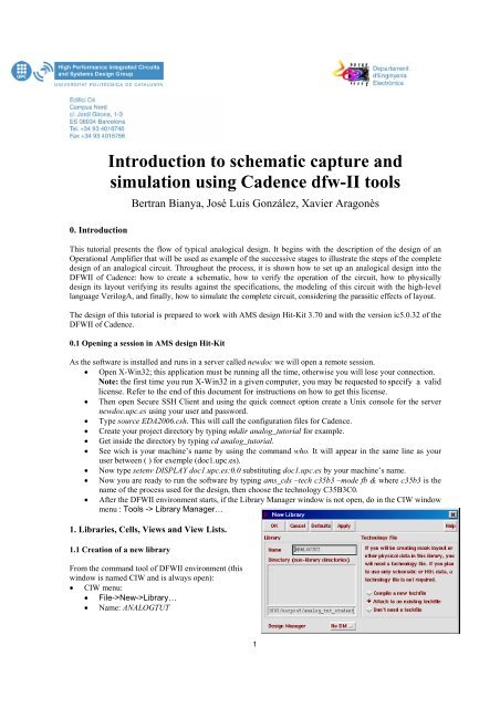
Attach to an existing technolgy file ONOKIn the window that will pop-up, select from the Technology Library list TECH_C35B3This library will be used to place all the new cells created along this tutorial.1.2 Adding and existing libraryAll the cells that will be created in this tutorial have been previously designed and they are contained, as solution,in an existing library. To add this library to the Library Manager tool, we have to use the Library Path Editor inthe following way:From the Library Manager window:Libray Manager menu: Edit->Library Path… Library: ANALOGTUT_SOL Path:$AMS_DIR/training/analog/ANALOGTUT File-> Save as... (do not changethe suggested path and file name,cds.lib; ignore the message "cds.libis not edit locked") File -> Exit (or Control+x)1.3 Libraries structure in Cadence DFWIIEach design and each project has their own Library. There we will import or create the different Cells that willperform the project and their corresponding Cellveiws.The libraries of Cadence are structured and mapped in a hierarchic tree. Each Library is associated to a rootdirectory, each Cell inside the Library is a subdirectory of the Library’s root directory and each Cell View is asubdirectory of the Cell’s subdirectory.The file cds.lib contains the physical locations of the libraries root directory and their logical name used inCadence. This file is automatically generated when AMS design kit is invoked, containing the native Cadencelibraries and the libraries of AMS design kit. Any library that we create will add a line to this file.In the Unix console you can type cat cds.lib and you will view the file content. You can find forexemple this lines for the predefined libraries:INCLUDE $AMS_DIR/artist/HK_ALL/env/cds.libDEFINE TECH_C35B3 $AMS_DIR/artist/HK_C35/TECH_C35B3DEFINE PRIMLIB $AMS_DIR/artist/HK_C35/PRIMLIBDEFINE IOLIB_3M $AMS_DIR/artist/HK_C35/IOLIB_3MAnd this lines for the libraries you have created and added:DEFINE ANALOGTUT /export/home/cursos2005/usrcad3/tutorial_analog/ANALOGTUTDEFINE ANALOGTUT_SOL $AMS_DIR/training/analog/ANALOGTUTDEFINE ANALOGTUT_STREAM /export/home/cursos2005/usrcad3/tutorial_analog/ANALOGTM2 Introduction to schematic capture and simulation using Cadence DFW-II

The libraries in Cadence can be visualized and set-up from the utility Library Manager. The following figureshows an example of this utility with the cells and the views for one of the cells (op_amp) of ANA_TUT library.In the next figure its equivalence to the file system structure is shown.1.4 The concept of View in CadenceAny cell can be described in several ways. In general we could group these ways in three cathegories: schematicdescription, behavioral description and physical description. Cadence uses one or more Views to describe acircuit. Each View is identified by a unique name previously defined. It is possible to create own names of views,but always we have the View type, which is a property added to the file that describes each View of the cell.For exemple each cell needs a symbol View to be instantiated in a higher level of hierarchy. A schematic Viewhas associated a symbol View, and a layout View (physical cell description) has associated an abstract View(physical symbol view) . These are the main views, but as it will be seen, there are variations to be able to usethem in different design contexts.There are many types of behavioral views, since there is one required for each of the different high-leveldescription languages. Digital behavioural views usually are named behavioural or functional, whereas theanalog behavioural views have a name associated to the language used to describe them. For example, theVerilogA descriptions are contained in views named ahdl.3

There are Views that contain the information necessary to simulate the cells. Behavioral descriptions can besimulated directly, but other cells need a particular view for each different simulator. These simulation views arenormally found only in the lowest level of the design hierarchy (devices, passives, sources, etc). A particular caseis the digital cells from standard cell libraries, which have a symbol View that is also used for simulationpurposes.The following table shows typical vies for a digital and a analog basic cell:Digital basic cellabstractabstract_mlvscmos_schlayoutmspssymbolAnalog basic celladsauCdsauLvseldoeldoDhsimhsimDhspiceSlayoutspectrespectreSsymbolFrom the point of view of the simulation process (specifically, from the netlister tool point of view) there arethree categories of views:Stopping views:These views are the primitive views necessary for the simulators. They contain the properties necessary to informto the netlist generation process how the information must be written in a specific component. These viewsusually have the same name that the simulator (Spectre, SpectreS, hspiceS, eldo, etc). As mentioned before, somebehavioral descriptions using, for example, Verilog, VHDL or VerilogA languages are also stop views. Forexample, the ahdl view is a stop view that will be simulated with the SpectreAHDL simulator, a subprogram ofthe SPICE-like simulator Spectre.Switching views:These views are intermediate levels of the design hierarchy and they will always contain instances to cells withother structural or stop views. The commonest structural view is schematic, that can contain basic elements likeresistors, capacitors or transistors, that will have a stop view (for example spectre) or other structural elementswith views of type schematic.The cmos.sch view is special a schematic view that appears in the digital cells to allow the transistor levelsimulation coexist with the logic simulation of the same cell.The views of type extracted are also structural, since they contain the devices and passive components extractedfrom layout of the circuit.Non simulation viewsSome views are not appropriate for simulation, like the physical design layout View. These views themselvescontain no useful information for any simulator but by applying some post-processing (the extraction ofparasitics and devices) they can be transformed into simulation views (for example, the extracted view).4 Introduction to schematic capture and simulation using Cadence DFW-II

1.5 View lists for simulation and analysisThe same design can be simulated in many different ways, if the proper views are available. For this reason it isnecessary to set up a process that specifies what view to use in each of the cases. The netlister selects theappropriate description of the circuit according to the type of simulation and the available view for each cell inthe hierarchy. This process is controlled by means of two view lists:Switch view list: this list defines the views that will be considered in the netlisting process. The order isimportant because it defines the order in which the available view for each cell will be analyzed.Stop view list: this list contains the stopping views according to the simulations that are selected to be used in theanalysis.The procedure of netlist generation is the following: the highest level of the hierarchy is analyzed first, lookingonly to the views that appear in the Switch view list in the order in which they are defined for the cells that itcontains. If a view for a cell is found then it is checked whether this view is in the Stop view list or not. If it isnot, the netlister descends a level into the hierarchy for that cell and iterates the process. If the view list analyzedfor a particular cell is found in the Stop view list, the information for the simulation is extracted from that viewand added to the netlist, stopping the hierarchical analysis for that cell. The process is completed when all thecells with stopping views have been visited and netlisted.Some examples of view lists set-ups for different types of simulations:a) Transistor level simulation (for pure analog designs):Switch view list: spectre schematicStop view list: spectreb) Transistor level simulation (for pure digital designs):Switch view list: spectre cmos_sch schematicStop view list: spectreIn this design, each cell having only a schematic view will be hierarchical traversed until the instanceswith a spectre View are found. Digital cells have a schematic view named cmos_sch instead ofschematic.c) Mixed signal simulation: analog section at transitor level / digital section at logic level:Switch view list: spectre symbol schematicStop view list: spectre symbolComparing with the previous case, the symbol View is placed first before schematic View. In this way, digitalcells will be first analyzed using its symbol View, which is also a simulation view (it is in the Stop view list).The relevance of the order used in the Switch view list can be explained using the following example.The basic analog components (resistors, transitory, etc.) have both a symbol View (used to instantiate thecomponents in the schematic view of the higher level) and a spectre View (used for simulation). Since the viewspectre is found first in the Switch view list and it is also found in the Stop view list, that will be the view used fornetlisting, and the symbol View will not be analyzed. Digital cells have no spectre view and their schematic viewis named cmos.schs. Therefore, the symbol View plays the same roll for digital basic cells that the spectre Viewfor basic analog components. This behavior also allows classifying the two sections of the design, since they willbe simulated using different simulators. All the spectre Views collected by the netlister will be assigned to theanalog partition and simulated by the SPICE-like simulator Spectre. All the symbol views of the digital cellscollected by the netlister will be assigned to the digital partition and simulated using Verilog or VHDL5

simulators. The signals that go from one domain to the other are implemented with interface elements thatperform the proper signal conversion.d) Transistor level simulation using the extracted layout:Switch view list: spectre extracted schematicStop view list: spectreThis is another example of the importance of the order. For a particular circuit it should be a schematicView that contains the circuit description. If the layout of this circuit has been completed, it is possible togenerate an extracted View that contains the transistor level circuit derived from the layout, including parasitics.If this is the circuit that has to be simulated, the extracted View must be placed before the schematic View in theSwitch view list.e) Behavioral simulation using ahdl models:Switch view list: spectre ahdl schematicStop view list: spectre ahdlIt is also possible to have a behavioral description of a circuit in addition to the circuit schematic. Thisbehavioral view will simulate much faster. If we want the netlister to select this view instead of the schematicView of the cell, we must place ahdl View before schematic View in the Switch view list. Since ahdl View is alsoa simulation view, it must be added to the Stop view list.Lets consider the following OpAmp circuit, where the following views are available:abstractahdlextractedlayoutschematicsymbolNext table shows the number of components and the simulation time for some of the previous simulationconfigurations.Smulation # components Simulation timea) Schematic 30 0,85 sd) Extracted 129 1,43 se) AHDL 9 0,35 s6 Introduction to schematic capture and simulation using Cadence DFW-II

2. Schematic capture and simulation:The first steps in this tutorial design flow are: firstly drawing the transistor level schematic of an operationalamplifier, secondly simulate it. The circuit used is the two stages operational amplifier described in the bookCMOS Analogue Circuit Design de Philip E. Allen y Douglas R. Holberg. The design goal is to achieve, with asimple circuit, a 1 MHz of bandwidth.The schematic of the circuit is composed of basic components (transistors, resistors and capacitors) from thePRIMLIB library. Follow the next steps:2.1 Creation of a new cell:CIW menu: File->New->Cellview… Library Name: ANALOGTUT Cell Name: op_amp View Name: schematic Tool: Composer-Schematic OKThe schematic editor Virtuoso opens.2.2 Schematic capture of the op_amp cell circuitUse the following figure to draw the schematic of the cell. The component sizes and values are listed in the tablebelow:Be careful when you put the transistors, the arrows must be in the same place and in the same direction. op_ampcircuit component sized and values7

Comp Library Cell View Parameter Comp Library Cell View Parameterw = 5µ w = 5µT1 PRIMLIB nmos4 symbol l = 3.05µ T2 PRIMLIB nmos4 symbol l = 3.05µng=1ng=1w = 100µ w = 200µT3 PRIMLIB nmos4 symbol l = 3.05µ T4 PRIMLIB pmos4 symbol l = 3.05µng=2ng=4w = 10µ w = 10µT5 PRIMLIB pmos4 symbol l = 10.05µ T6 PRIMLIB pmos4 symbol l = 10.05µng=1ng=1w = 50µ w = 50µT7 PRIMLIB nmos4 symbol l = 3.05µ T8 PRIMLIB nmos4 symbol l = 3.05µng=4ng=4R = 465K C = 3.466pR1 PRIMLIB rpoly2 symbol l = 4000µ C1 PRIMLIB cpoly symbol w = 100µw = 0.7µl = 40µTo add a new component use the toolbar buttonor press key iUse the table information to fill the forms that appearassociated to each component. The placement andorientation of the componets can be varied using the buttonson the form Rotate, Sideways and Upside Down.Other useful comands for editing the schematic are:Adding a wire (to conect two nodes of the circuit) Add->Wire (narrow) (or type w)Adding a pin (to place an external input or output) Add->Pin…In this case, a form appears with the options of the pin,where the pin name and directino should be set:Once the circuit drawing has been completed, it is necessary to check it. Any connectivity error or design ruleviolation is checked during this step. Additionally, the circuit netlist is automatically generated from the drawingeach time the schematic is checked in the Virtuoso editor window. To check the schematic do:Virtuoso Schematic Editor menu Design->Check and Save8 Introduction to schematic capture and simulation using Cadence DFW-II

2.3 Generation of the symbol View from the op_amp schematic ViewIt is necessary to create a symbol that will represent the schematic we have just created in higher levels of thedesign hierarchy. To do so, follow the next steps: From the Virtuoso SchematicEditor window that contains thecircuit schematic View Design->Create Cellview->From Cellview… Library Name: ANALOGTUT Cell Name: op_amp From View Name: schematic To View Name: symbol OKDuring this process, a new window opens with the options of the symbol generation where the location of theterminals is specified (top, bottom, left, right). After pressing OK in this new window the Virtuoso SchematicEditor opens containing an automatically generated drawing of op_amp cell symbol. This default drawing can beedited and modified, until it resembles the figure below:2.4 Creation of a testbench to simulate the op_amp circuitThe recently completed circuit is an analog cell with input, output and power supply pins. If we want to simulateit, we need to add the appropriate stimulus to the inputs and provide the biasing requiring for the circuit. This isdone by connecting signal sources to the input and biasing pins of the cell in a higher level of the designhierarchy. This new cell will contain an instance to the op_amp Cell along with the signal and biasing sources.The output of the operational amplifier will also be terminated to provide a realistic loading.From CIW menu: File->New->Cellview… Library Name: ANALOGTUT Cell Name: op_amp_test View Name: schematic Tool: Composer-Schematic OK9

In the new Virtuoso Schematic Editor window that appears draw the schematic of the testbench as shown in thefigure below. The sources and other components are taken from the analogLib Cadence library. Use theaccompanying table to set the components values and parameters.To help in the simulation analysis, it is recommended to add meaningful names to the wires:Add->Wire Name…It is possible to use the same form to give several names. Just write the wire names separated by blanks andthen press the tab key to start the placement of the wire names.Please be really careful when you draw a schematic any wrong wire connected will produce strange results.Comp Library Cell View Parametergnd analogLib gnd symbol -V0 analogLib vdc symbol vdc = 3.3 VV1 analogLib vdc symbol vdc = 1.65 VV2 analogLib vdc symbol acm = 1 VC0 analogLib cap symbol cap = 10p FR0 analogLib res symbol res = 1M ohmI3 ANALOGTUT op_amp symbol -Schematic drawing and component values for op_amp_test Cell.2.5 Pre-layout simulation of the circuitIn this section of the tutorial, the circuit is simulated at transistor level to verify the circuit specifications. Thesimulation consists of an AC analysis to measure the op_amp cell open loop gain and phase responseagainst frequency.Follow the next steps:10 Introduction to schematic capture and simulation using Cadence DFW-II

2.5.1 Open the schematic:If the simulation test bench (op_amp_test cell, schematic view) is not currently open it can be oponed either bydouble clicking with the mouse left button over its name in the Library Manager or by using the CIW menu.2.5.2 Analog Circuit Design Environment set up:The simulation will be performed from a window named Affirma Analog Circuit Design Environment,previously known as Analog Artist. The simulation environment is call from the Virtuoso Schematic Editorwindow that contains the cell schematic view, in our case the op_amp_test cell schematic view.Tools -> Analog EnvironmentThe simulation environment window opens indicating the simulated cell in the Design field. The next step is theconfiguration of the Simulator parameter using various menus and options of the simulation environmentwindow.The default Simulator engine is Spectre, so we don’t need to modify this. However, it is very recommended tocheck all the options form the Setup menu, specially the following:Localization of the simulation models for the basic components (Setup->Model Libraries…)Simulator engine and simulation directory (Setup->Simulator/Directory/Host…), the defaultfolder for simulations is going to be Sim inside your project folder.2.5.3 Simulation environment set-up:The following analysis options have to be selected in order to perform an AC simulation:Analysis -> Choose…11

Finally, alter pressing OK en in the analysis option tab, the simulation environment window should look like this:The simulation set-up is saved in a file named the ‘state’ of the simulation. There can be several simulation setupsfor the same schematic. This allows recovering the simulation environment set-up in subsequent sessions. Tosave the current set-up (‘state’) of the simulation environment follow the next steps:12 Introduction to schematic capture and simulation using Cadence DFW-II

Session -> Save State…The state name chain be choosen arbirtraryly but it is recommended to use meaningfull names. The states arestored in a hiden subdirectory named .artist_states, in the user home diretory, independently of theDFWII working directory.2.5.4 Run the simulation:Once the various simulation options have been selected, the simulation can be started in the following way, fromthe simulation environment menu: Simulation -> Run (or by clicking the green light button in the toolbar )A new text window pops-up showing simulation messages with information about the circuit and the simulationsteps. The simulation is finished if yu can see at the end the total time required for de analysis.2.5.5 Simulation results analysis:After the simulation ends, the results are stored in files and subdirectories under the simulation directoryspecified during the set-up step. We are interested in the open-loop gain and the phase response. We also want toobtain the bandwidth and the phase margin. These quantities are calculated from the simulation results. Thecalculator tool will be used for this purpose. From the simulation environment window the calculator tool is runin the following way:Tools -> CalculatorThe calculator operates on current and voltage waveforms saved in the simulation results file after the simulation.These waveforms are selected by clicking at the corresponding nodes or terminals in the schematic circuit.Therefore, we need the Virtuoso Schematic Editor window opened simultaneously with the simulationenvironment. Always look at the bottom part of the schematic window to check if there is some node selectioncommand running and waiting for a response. To cancel these commands just press ESC key. The calculator usesRCL notation and stores intermediate results in a stack. To visualize this stack just press the button DisplayStack on the calculator window. Now let’s practice with the calculator tool.Open loop gain measurement- Click vf (this means voltage against frequency, the result of AC analysis)- Select in the schematic the following nodes in the order listed: out, inp, inn, you should not press enterafter each selection (the calculator window should look like this):13

- In the calculator press first ‘-‘ and next ‘/’. Finally press the dB20 button. The window should looklike these after the previous sequence of operations:- The button plot draws the calculated expression, if it is a waveform, that is found at the first level ofthe stack (note that if the expression results is a number, the button print should be used instead of plotto print the numeric result in a new window that will pop-up).14 Introduction to schematic capture and simulation using Cadence DFW-II

If you don’t get this exactly plot, go to the op_amp and op_amp_test schematics and pay attention if you havemade any mistake drawing the circuits.Phase noise responseProceed in a similar way as before to get the following expression in the first level of the calculatorstack:Press the plot button to draw the new curve. Now the Waveform window shows two overlaped curves.To place each curve in a different panel use the following option of the Waveform window menu:- Axes->To StripTittles and labes can be added from the annotaion menu (see next page for an example):- Annotation->Title-3dB Cut-off frequency, Phase marginThese two measurements are numeric results, not waveforms. They can be calculated with the followingexpressions using the calculator:bandwidth(VF(“/out”)/(VF(“/inp”)-VF(“/inn”)),3,”low”)The result can be visualized by pressing the PRINT button. The -3db cut-off frequency should be 15.9Hz. The phase margin is calculated with the following expression:phaseMargin(VF(“/out”)/(VF(“/inp”)-VF(“/inn”)))It is the difference between the phase 180º and the phase equivalent to the frequency when the gain isunity. It should result in approximately 50º.This figure shows the final aspect that should have the Waveform window after plotting the results.15

2.5.6 Saving the results:The simulation results (not the waveforms drawn) can be stored to compare them with further simulations. Thisis accomplished by using the following command, from the simulation environment window menu:Results -> Save…It is recommended to add a comment to easily identify the saved results. These results will always be associatedto the schematic cell that has been simulated.16 Introduction to schematic capture and simulation using Cadence DFW-II

3. Analog behavioural modeling and simulationIn the previous section you have completed a transitor level design of an operation amplifier and verified itsperformance through simulation. In this cell has to be used in a more complex design it is useful to have asimpler model of the cell that would simulate faster than the transitor level circuit. One possible option is tocreate a behavioral view of the same cell using VerilogA language to describe the function of the circuitcontaining only the necessary details for system-level analysis.3.1 AHDL model generationFrom the simulation results of the previous section, it has been shown that the operation amplifier has a low-passfrequency response with two poles and one zero. Since there is a dominant pole the behaviour of the circuit canbe modeled with a simple first order RC circuit and a gain function.Follow the next steps to create the cell view and write the VerilogA model:3.1.1 AHDL view creation CIW menu: File->New->Cellview… Library Name: ANALOGTUT Cell Name: op_amp View Name: veriloga Tool: VerilogA Editor OKThere is an alternative way to do this, from the schematic view of the circuit. If we use this option, the inputand output names will be added automatically to the heading of the VerilogA model:Virtuoso Scematic menú: (editando la vista schematic del circuito que queremos modelar) Design->Create Cellview->From Cellview… Library Name: ANALOGTUT Cell Name: op_amp From View Name: schematic To View Name: veriloga Tool: VerilogA Editor OKAfter clicking OK a text editor window will open (emacs) 1 .3.1.2 VerilogA model creationUse the text editor to enter the following model. You cannot just paste the code, you must write it or modify thetemplate (you can also create a file verliloga.va file with this code and by ftp put it in the ../op_amp/verlioga/folder… the problem is that when you will create the cell the code will have incorrect characters that you willhave to fix):// VerilogA for ANALOGTUT, op_amp, veriloga`include “constants.h”`include “discipline.h”// Pin declarationsmodule op_amp(OUT, INN, INP, VDD, VSS);1 It a text editor does not open, this is probably because the EDITOR variable in your .csh configuration file points to vi, nanoor other editors that are opened in the console window.17

output OUT;input INN,INP,VDD,VSS;electrical OUT,INN,INP,VDD,VSS;// params and variablesparameter real cut_off_frequency = 50.0;parameter real gaindB = 100;real c0;real r0;real gain;// internal nodeelectrical internal_node;analog begin// initial calculations@ (initial_step or initial_step(“dc”)) beginr0 = 1/(2*3.141592654*cut_off_frequency*10e-6);gain = pow(10, (gaindB/20));endc0 = 10e-6; // always et to 10uV(internal_node)

3.2.2 Simulation environment set-upThe simulation set-up was previously store in the ‘state’ file, so we don’t need to repeat all the configurationsteps. Just load the previous ‘state’ after starting the simulation environment:Session -> Load State… (Fill in the form as shown bellow, selecting the ‘state’ name used tosave the simulation set-up in the previous section).It is imporatant to check that a DC analysis will be also performed to save the static operating point of the circuit:Analyses -> Choose…Check the DC box.The form should look like this:You have also to change the Switch View List to usethe ahdl view:Setup->Environment…Fill in the form as shown in thenext figure:19

Since the VerilogA model was parameterised, you have to assign the correct values to the bandwith and gainparameters. You can obtain these numbers from the simulation done at transitor level in the previos section: the -3dB cut-off frequency (15.9 Hz) and the gain in dB (105.5 dB). These parameters are defined for the op_amp cellinstante container in the op_amp_test testbench cell. This can be done as follows:In the Virtuoso Schematic Editor window (schematic view of op_amp_test cell): Select the op_amp symbol Edit->Properties->Objects…IN the form that pops-up, press the item list named Use Tools Filter20 Introduction to schematic capture and simulation using Cadence DFW-II

Fill in the model parameters as shown in the figure below:Finally, ckeck and save the changes done in the op_amp_test schematic.Design->Check and Save3.2.4 Simulation and resultsYou have to follow the same steps of sub sections 2.5.4 y 2.5.5. After the simulation ends you have to plot thephase response and open-loop gain. They should look like the following figure (next page):Now, the bandwidht and phase margin measurments should be, approximatelly, 16 Hz y 90 degrees, respectively(the large difference in the latter is due to the first order RC model used that has a sinble pole). Thesemeasurments are obtained using the following expressions in the calculator:bandwidth(VF(“/out”)/(VF(“/inp”)-VF(“/inn”)),3,”low”)phaseMargin(VF(“/out”)/(VF(“/inp”)-VF(“/inn”)))21

3.2.5 Circuit level and AHDL behavioural modelcomparisonWe saved the simulation results for the transistorlevel description of the operational previously. Now,we can load these results and plot them on top of theAHDL results we have just obtained and compareboth. This is done in the following way:In the simulation environment menu:Results->Select…Select the schematic-save name and press OKNow, any expression in the calculator applies to the loaded results instead of the last simulation run results. Plotthe same expressions as before (open loop gain and pahse response).NOTE: If the Waveform window was closed for some reason, only the new curves will be plotted. If you want toplot again the AHDL simulation results, you have to select the result file name schematic and repeat theprocess. This result name corresponds always with the last simulation run results.The several waveform can be grouped to place the same type of mesurement in the same panel. Use theWaveforom window menu tool -Axes->To Strip. This will creat four panesl. Waveforms can be moved formone panel to the other by draggin and droping the curve with the mouse. You should obtain a Waveform windowsimmilar to the figure below:22 Introduction to schematic capture and simulation using Cadence DFW-II

END of the tutorial. If you have troubles be patient and pay attention to all the steps.______________________________How to provide a valid license to X-Win 32:1. In the X-Win32 License Wizard, select "Network (Floating)". OK.2. Open a web browser and go to http//deenord.upc.es3. Click on "Sistemas windows XP", then on "Licencias de software" (on the left bar); then on "Licencia de Xwin32"4. Copy the text of the license to the W-Win32 window that asks for it. Next. Finish23