- Page 1 and 2: Comprehensive System Identification
- Page 3 and 4: APROVAL PAGETITLE:AUTHOR:Comprehens
- Page 5 and 6: ACKNOWLEDGMENTSThe author would lik
- Page 7 and 8: 3.4.4 Magnetometer Identification..
- Page 9 and 10: LIST OF FIGURESFigure 1.1 - Land Wa
- Page 11 and 12: Figure 3.48 - Magnetometer Depictio
- Page 13 and 14: CHAPTER 1 - INTRODUCTION AND MOTIVA
- Page 15 and 16: The vehicles examined within the sc
- Page 17 and 18: tunnel testing to study the charact
- Page 19 and 20: Figure 1.8 - Helicopter Body Axes S
- Page 21 and 22: GPSRate GyrosAccelerometersIMUInner
- Page 23 and 24: CHAPTER 2 - METHODS AND TECHNIQUES2
- Page 25 and 26: 2.2.1 Flight Test TechniquesThere a
- Page 27 and 28: manufacturer specifications are mod
- Page 29: 3.2 Bare-Airframe IDThe bare-airfra
- Page 33 and 34: ⎧ p⎫⎪ ⎪y = ⎨q⎬⎪ r ⎪
- Page 35 and 36: Table 3.4 - OAV DERIVID Identified
- Page 37 and 38: The identified state-space model yi
- Page 39 and 40: Better sensors, at higher sampling
- Page 41 and 42: Figure 3.3 - Yaw response frequency
- Page 43 and 44: Figure 3.4 shows that even though t
- Page 45 and 46: It can be seen that the Aerovironme
- Page 47 and 48: 3.2.2 Allied Aerospace MAVFlight te
- Page 49 and 50: 30MAGNITUDE(DB)-10-50250PHASE(DEG)5
- Page 51 and 52: A 0th/2nd order transfer function i
- Page 53 and 54: Figure 3.12 shows the same for the
- Page 55 and 56: Techsburg) the pitching moment resp
- Page 57 and 58: Table 3.11 shows that all of the di
- Page 59 and 60: Figure 3.14 shows how increasing th
- Page 61 and 62: the duct, the effects of the man ne
- Page 63 and 64: ft-lbMu PLATFORM= 5.11ftsecThis dim
- Page 65 and 66: apparent that the size of the duct
- Page 67 and 68: adequate way to characterize the di
- Page 69 and 70: actuators varied in size, weight, c
- Page 71 and 72: It is noticeable from the figure th
- Page 73 and 74: Table 3.17 - Actuator Calibration F
- Page 75 and 76: Figure 2.1 shows an example frequen
- Page 77 and 78: The test matrix is provided as Tabl
- Page 79 and 80: frequency response curves shown in
- Page 81 and 82:
Table 3.22 shows that for the first
- Page 83 and 84:
The time delays all seemed to be ar
- Page 85 and 86:
400035003000250020001500y = -13429x
- Page 87 and 88:
higher data rates, and tighter tole
- Page 89 and 90:
esponse and the response obtained f
- Page 91 and 92:
The time histories show that the ou
- Page 93 and 94:
Figure 3.31 - Magnitude Comparison
- Page 95 and 96:
Performing the frequency response a
- Page 97 and 98:
Results from STI utilizing the exac
- Page 99 and 100:
The fact that the rate saturated du
- Page 101 and 102:
Table 3.23 for the maximum rates an
- Page 103 and 104:
Verification of the identified mode
- Page 105 and 106:
from testing (3.22), it was found t
- Page 107 and 108:
3.4.1 Accelerometer IdentificationM
- Page 109 and 110:
Figure 3.43 shows that gyros were m
- Page 111 and 112:
5 meter circle centered about the t
- Page 113 and 114:
Figure 3.46 shows the modeled fluct
- Page 115 and 116:
Figure 3.49 - Pressure Altimeter Mo
- Page 117 and 118:
Figure 4.1 - Simulink MAV ModelFigu
- Page 119 and 120:
Figure 4.3 - Simulink Sweep Generat
- Page 121 and 122:
cause a pitching moment to be exert
- Page 123 and 124:
Figure 4.6 - Cross Control Decoupli
- Page 125 and 126:
⎡ Lp Lq Lr Lu Lv Lw0 0 0⎤⎢MpM
- Page 127 and 128:
It can be seen right away that the
- Page 129 and 130:
Figure 4.8 shows that the coherence
- Page 131 and 132:
CHAPTER 5 - CONCLUSIONSThe need for
- Page 133 and 134:
6. Mettler, B., Tischler, M. B., an
- Page 135 and 136:
Appendix AOAV Proposal VehicleIdent
- Page 137 and 138:
DS8417 - 5V- 125 -
- Page 139 and 140:
HS512MG - 5V- 127 -
- Page 141 and 142:
DS368 - 5V- 129 -
- Page 143 and 144:
94091 - 5V- 131 -
- Page 145 and 146:
CS-10BB - 5V- 133 -
- Page 147 and 148:
Appendix CActuator Generated Transf
- Page 149 and 150:
DS8417 - 100% - 5V- 137 -
- Page 151 and 152:
DS8417 - 100% - 6V- 139 -
- Page 153 and 154:
HS512MG - 100% - 5V- 141 -
- Page 155 and 156:
HS512MG - 100% - 6V- 143 -
- Page 157 and 158:
DS368 - 100% - 5V- 145 -
- Page 159 and 160:
DS368 - 100% - 6V- 147 -
- Page 161 and 162:
94091 - 80% - 5V- 149 -
- Page 163 and 164:
94091 - 80% - 6V- 151 -
- Page 165 and 166:
CS-10BB - 100% - 5V- 153 -
- Page 167 and 168:
CS-10BB - 100% - 6V- 155 -
- Page 169 and 170:
Appendix DActuator Time Domain Veri
- Page 171 and 172:
94091 5V94091 6V- 159 -
- Page 173 and 174:
DS368 5VDS368 6V- 161 -