- Page 1 and 2:
Contents1 Course Administration 42
- Page 3 and 4:
10 Regression 20210.1 Introduction
- Page 5 and 6:
Resource PageDepartment of Mathemat
- Page 9 and 10:
3 Data and Study Designs3.1 Basic d
- Page 11 and 12:
Parameter• Parameter: Fixed numbe
- Page 13 and 14:
TypesDiscrete - can put in one-to-o
- Page 15 and 16:
- How do geologists know?- Sediment
- Page 17 and 18:
Source: skyscrapercity.comSampling
- Page 19:
- 1 in 3.8 million - 3.8 million di
- Page 23 and 24:
Important designs• Completely ran
- Page 25 and 26:
B. Randomised control - of all chil
- Page 27 and 28:
- Reason why observational studies
- Page 29 and 30:
Things that go wrong• Even the be
- Page 31 and 32:
4 ProbabilityFred’s DayFred awoke
- Page 33 and 34:
• The event that the mouse we tra
- Page 35 and 36:
Blood donor example - Multiplicatio
- Page 37 and 38:
Fair Die Example• A fair die is t
- Page 39 and 40:
Tree diagram rules• Add Verticall
- Page 41 and 42:
Tree Diagrams - Independent Stages0
- Page 43 and 44:
Dependent Stages• Andrew, John an
- Page 45 and 46:
0.90BBiopsy +ve (true positive)0.00
- Page 47 and 48:
Calculating Probabilities• Estima
- Page 49 and 50:
4.3 Random VariablesRandom Variable
- Page 51 and 52:
Calculating the Variance• The sam
- Page 53 and 54:
Examples• Consider a data set XX
- Page 55 and 56:
Combining 2 Random Variables• If
- Page 57 and 58:
Fred’s DayShould Fred be worried
- Page 59 and 60:
Now using the complementary event r
- Page 61 and 62:
Mean of Binary DistributionThe mean
- Page 63 and 64:
• Mean number of successes• Var
- Page 65 and 66: Using the Formulan = 3, x = 2, π =
- Page 67 and 68: • A probability less than 0.05 is
- Page 69 and 70: Endangered bird egg example solutio
- Page 71 and 72: RELATIVE FREQUENCY HISTOGRAMNormal
- Page 73 and 74: Finding Areas Under the Curve• In
- Page 75 and 76: • Find P r(−1 < Z < 1.64)pnorm(
- Page 77 and 78: INVERSE PROBLEMS USING R-COMMANDER
- Page 79 and 80: CALCULATING PROBABILITIESAssume tha
- Page 81 and 82: CONTINUITY CORRECTION• Normal pro
- Page 83 and 84: Sample size = 10Consider the situat
- Page 85 and 86: ConclusionWhat conclusion would you
- Page 87 and 88: 10%5.5 6.0 6.5 7.0 7.5 8.0 8.5XWe k
- Page 89 and 90: 6 Sampling Distributions and Estima
- Page 91 and 92: DERIVATION IWe can think of the sam
- Page 93 and 94: Solution IIPr(X > 172) = 1 - pnorm(
- Page 95 and 96: qnorm(0.975) as 2.5% of the area is
- Page 97 and 98: 6.2.1 Sample Size CalculationEXAMPL
- Page 99 and 100: The 99% Confidence IntervalThe 99%
- Page 101 and 102: 6.3 Comparing Two SamplesCOMPARING
- Page 103 and 104: THE POOLED VARIANCEIf the variances
- Page 105 and 106: SOLUTION - Calculating the confiden
- Page 107 and 108: Confidence Interval for raw dataTo
- Page 109 and 110: = 6.6 ± 24.6That is, -18.0 < µ in
- Page 111 and 112: STANDARD DEVIATIONIf P = X n : σP
- Page 113 and 114: 6.4.2 Sample Size CalculationEXAMPL
- Page 115: Fred for MayorFred has decided to t
- Page 119 and 120: 7 Hypothesis TestingFred’s Parkin
- Page 121 and 122: • If the standard deviation is un
- Page 123 and 124: Find the p-value:Pr(Z < -2.78)=0.00
- Page 125 and 126: EXAMPLE THREE (B) - HYPOTHESIS TEST
- Page 127 and 128: 7.4 Hypothesis Test Difference Two
- Page 129 and 130: 7.5 Interpreting the p-valueINTERPR
- Page 131 and 132: (a) Mean difference = 40, confidenc
- Page 133 and 134: INCONCLUSIVE CONFIDENCE INTERVALSNo
- Page 135 and 136: ERROR TYPESAccept RejectH 0 True Co
- Page 137 and 138: Part IIFred sets the hypothesis out
- Page 139 and 140: 8 Contingency TablesFred’s Garden
- Page 141 and 142: • For the purpose of this course
- Page 143 and 144: What can we do with this informatio
- Page 145 and 146: So in our swimming example:• Odds
- Page 147 and 148: Confidence interval for relative ri
- Page 149 and 150: So the confidence interval is given
- Page 151 and 152: ln(OR) ± 1.96 × s.e.(ln(OR))−0.
- Page 153 and 154: 8.6 Chi Square Test for Contingency
- Page 155 and 156: • We can continue to calculate th
- Page 157 and 158: Some notes on χ 2• Maximum power
- Page 159 and 160: Admit Decline TotalMale 490 [449.2]
- Page 161 and 162: • ¯x = Σn ix iN = 2174868 = 2.5
- Page 163 and 164: Fred’s GardenSo Fred recorded the
- Page 165 and 166: Since 1 is excluded there is strong
- Page 167 and 168:
AdoptiveBiological Parents’ SESPa
- Page 169 and 170:
EXAMPLE: Cuckoo Egg LengthsCompare
- Page 171 and 172:
9.1.3 F DistributionF DISTRIBUTION
- Page 173 and 174:
EXAMPLE20 children allocated random
- Page 175 and 176:
RESIDUAL MEAN SQUARE (s 2 e)Group A
- Page 177 and 178:
Notes• Degrees of freedom are 15
- Page 179 and 180:
9.4 Two factor ANOVATWO FACTOR ANOV
- Page 181 and 182:
• Conclusion:There is some eviden
- Page 183 and 184:
NOTES• We need to give two parts
- Page 185 and 186:
CONFOUNDING VARIABLEPotential varia
- Page 187 and 188:
INTERACTIONA significant interactio
- Page 189 and 190:
CALCULATING INTERACTION EFFECTInter
- Page 191 and 192:
• Convert numerical group names i
- Page 193 and 194:
• The city effect is not the same
- Page 195 and 196:
General Level SS = 18 x ( 26418 )2=
- Page 197 and 198:
Calculating the Test StatisticTest
- Page 199 and 200:
And finally he needed to work out t
- Page 201 and 202:
2. H 0 The mean IQs of children wit
- Page 203 and 204:
He sent her some data resulting fro
- Page 205 and 206:
More complex relationships• Look
- Page 207 and 208:
Equation for a straight line• We
- Page 209 and 210:
Instead use method of least squares
- Page 211 and 212:
• Compute interceptˆβ 0 = ȳ
- Page 213 and 214:
An example - Analysis of variance
- Page 215 and 216:
Normality Assumption P-P plotPP Plo
- Page 217 and 218:
2nd Residual Plot FAILStandardized
- Page 219 and 220:
n∑(x i − ¯x) 2 = 23485.35i=1x
- Page 221 and 222:
Prediction Interval• We can find
- Page 223 and 224:
• A confidence interval estimates
- Page 225 and 226:
Correlation• The correlation coef
- Page 227 and 228:
Non-linear Correlation• In the pr
- Page 229 and 230:
• Therefore r 2 = 0.8931, so 89.3
- Page 231 and 232:
• where ˆβ 0 , ˆβ 1 , ˆβ 2
- Page 233 and 234:
• Age alone.ŷ = 5.0688 + 0.0359a
- Page 235 and 236:
Dummy variables in lung capacity ex
- Page 237 and 238:
Height Vs Lung Capacity• From bef
- Page 239 and 240:
Three variable modelTest of the Hyp
- Page 241 and 242:
• Giving a confidence interval of
- Page 243 and 244:
Extra sum of squares modelSource of
- Page 245 and 246:
●●LinearModel.2res−2 −1 0 1
- Page 247 and 248:
• At this stage the ages have bee
- Page 249 and 250:
Multiple Regression• Now lets per
- Page 251 and 252:
Multiple Linear Regression GraphTre
- Page 253 and 254:
Source of variation SS DF MS FRegre
- Page 255 and 256:
p1−p = expβ 0 + β 1 x 1 + . . .
- Page 257 and 258:
• logit = −1.674 + 1.841x 1Logi
- Page 259 and 260:
• OR = 6.98 (1.524,27.987)• The
- Page 261 and 262:
Example• The adjusted OR and CI w
- Page 263 and 264:
Next Fred calculated the β 1 :n∑
- Page 265 and 266:
This gives a confidence interval of
- Page 267 and 268:
ATools for assignmentsCommon Mistak
- Page 269 and 270:
Correct Approachå Evaluate 1.9
- Page 271 and 272:
BSummary of Formulae1. Normal Distr
- Page 273:
Estimate df (ν) Multiplier Standar