Design of a Hybrid Positioner-Fixture for Six-axis Nanopositioning ...

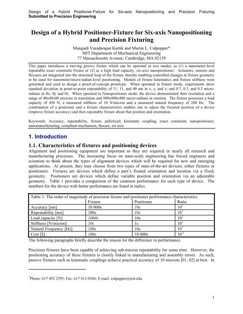
Design of a Hybrid Positioner-Fixture for Six-axis Nanopositioning and Precision FixturingSubmitted to Precision EngineeringDesign of a Hybrid Positioner-Fixture for Six-axis Nanopositioningand Precision FixturingMangudi Varadarajan Kartik and Martin L. Culpepper*MIT Department of Mechanical Engineering77 Massachusetts Avenue; Cambridge, MA 02139This paper introduces a moving groove fixture which can be operated in two modes; as (1) a nanometer-levelrepeatable exact constraint fixture or (2) as a high load capacity, six-axis nanopositioner. Actuators, sensors andflexures are integrated into the structural loop of the fixture, thereby enabling controlled changes in fixture geometryto be used for nanometer/micro-radian-level positioning. Models of fixture kinematics and fixture stiffness weregenerated and used to design a proof-of-concept prototype. When operated in fixture mode, experiments showstandard deviation in point-to-point repeatability of 11, 11, and 40 nm in x, y, and z; and 0.7, 0.3, and 0.3 microradiansin x, y and z. When operated in Nanopositioner mode, the device demonstrated 4nm resolution and arange of 40x40x80 microns in translation and 800x800x400 micro-radians in rotation. The fixture possesses a loadcapacity of 450 N, a measured stiffness of 10 N/micron and a measured natural frequency of 200 Hz. Thecombination of a positioner and a fixture characteristics enables one to adjust the fixtured position of a device(improve fixture accuracy) and then repeatably fixture about that position and orientation.Keywords: Accuracy, repeatability, fixture, palletized, kinematic coupling, exact constraint, nanopositioner,nanomanufacturing, compliant mechanism, flexure, six axis1. Introduction1.1. Characteristics of fixtures and positioning devicesAlignment and positioning equipment are important as they are required in nearly all research andmanufacturing processes. The increasing focus on nano-scale engineering has forced engineers andscientists to think about the types of alignment devices which will be required for new and emergingapplications. At present, they may choose from two types of state-of-the-art devices; either fixtures orpositioners. Fixtures are devices which define a part’s fixated orientation and location via a fixed,geometry. Positioners are devices which define variable position and orientation via an adjustablegeometry. Table 1 provides a comparison of the common performance for each type of device. Thenumbers for the device with better performance are listed in italics.Table 1: The order of magnitude of precision fixture and positioner performance characteristicsFixture Positioner RatioAccuracy [nm] 10 000s 10s 10 3Repeatability [nm] 100s 10s 10 1Load capacity [N] 1000s 10s 10 2Stiffness [N/micron] 10s 1s 10 1Natural Frequency [Hz] 100s 10s 10 1Cost [$] 100s 10 000s 10 -2The following paragraphs briefly describe the reason for the difference in performance.Precision fixtures have been capable of achieving sub-micron repeatability for some time. However, thepositioning accuracy of these fixtures is closely linked to manufacturing and assembly errors. As such,passive fixtures such as kinematic couplings achieve practical accuracy of 10 microns [01, 02] at best. In* Phone: 617 452 2395; Fax: 617 812 0384; E-mail: culpepper@mit.edu1

Design of a Hybrid Positioner-Fixture for Six-axis Nanopositioning and Precision FixturingSubmitted to Precision Engineeringcontrast, the active adjustment capability of positioners enables them to achieve tens of nanometersaccuracy and repeatability.The structure of passive fixtures is not constrained by the need to change geometry; therefore they may bedesigned with emphasis on high load capacity. The geometry of positioners must be variable and so theirstructures require bearings and joints which are orders of magnitude less stiff than the continuousstructure of a fixture. High stiffness is importance as it improves the disturbance rejection capabilities ofa machine. For instance, errors caused by external forces and vibrations generally decrease as stiffnessincreases.The improved stiffness characteristics of fixtures are in-part responsible for their higher naturalfrequencies. In contrast, positioners have lower natural frequencies because they include the additionalweight of actuation components and they often incorporate high-performance, low-stiffness joints orbearings. In the end, the cost of active elements, precision bearings and the need for precision assemblyof mechanisms-actuators-bearings make the cost of positioners higher than those of passive fixtures.The preceding discussion demonstrates the difficulties which must be overcome to make either devicehave the desirable characteristics of both devices. This begs the question, “Might we be able to somehowcombine the concepts of the fixture and positioner in a way which enables us to obtain the goodcharacteristics of each device and none of the bad?1.2. Conceptual approaches to integrating fixture and positioner technologyOne might attempt to synthesize a design in which the functional and physical characteristics of thefixture and positioner devices remain separated and the devices are then added in series or parallel. Froma positioning perspective, it would be sufficient to put the two devices in series (e.g. integrate a precisioninterface within the stage of a positioner). A part could be roughly aligned using the fixture and thenaccurately oriented and positioned using the positioner. Unfortunately, in this serial configuration thefixture and positioner would experience the same loading. As such, the cost, stiffness, load capacity anddynamic characteristics of this concept would at best approach those of the positioner. On the other hand,the parallel addition of a fixture and positioner is inappropriate as this would yield an over constraineddesign containing redundant kinematic chains.A different conceptual approach is required. Toward this end, we have developed a conceptual model andsupporting parametric models for a hybrid positioner-fixture (HPFs). The HPF incorporates precisionflexure bearings, exact constraint elements and actuators/sensors. The combination of these elementsenables the HPF to achieve passive repeatability of tens of nanometers and active correction of alignmenterrors over a range of tens of microns and hundreds of micro-radians. The key in this approach is to usethe capability of flexures to possess high stiffness in directions/orientations and low stiffness in 6-directions/orientations. This allows us to use flexures to simultaneously provide position adjustment in 6- directions and constraint in directions. In this work, the flexure bearings are incorporated into thestructural loop of the HPF such that they enable:(1) Positioning: The flexure bearing’s directions of high compliance are arranged parallel to the directionsin which we wish to actuate. These directions are laid out so that they do not have a detrimental effect onthe HPF stiffness when a high-stiffness actuator is used in parallel with the flexure.(2) Fixturing: The flexure bearing’s directions of high stiffness and high load capacity are aligned withthe vectors of force transmittal through the fixture’s structural loop, thereby enabling high load capacityand stiffness.2

Design of a Hybrid Positioner-Fixture for Six-axis Nanopositioning and Precision FixturingSubmitted to Precision Engineering1.3. Contents of this paperIn this paper, we describe the conceptual modeling of HPFs and how they may be parametricallymodeled. Experimental results are used to demonstrate the accuracy of the parametric models, thecapability of the HPF to act as a six-axis positioning device (six-axis displacements), and its capability toact as a positioner (accuracy and repeatability).2. Linking the characteristics and performance of fixtures andpositioners2.1. Analogy between constraints in fixtures and positioning mechanismsThe fundamental difference between fixtures and positioners is their respective static and variablegeometric/kinematic characteristics. Fixtures ideally have static structures while the structure ofpositioners is comprised of geometrically variable mechanisms. Any attempt to acquire the desirablecharacteristics of both devices must start with an effort to link the characteristics of a fixture’s structureand a positioner’s mechanisms. For small motions, it can be shown that exact constraint fixtures arekinematically equivalent to parallel mechanisms [01]. For example, the right side of Fig. 1 shows howthe 6 ball-groove constraints (2 per ball groove joint x 3 grooves) form the same arrangement ofconstraints that exist in a Stewart-Gough platform.Ball far-field pointConstraintGroove far-field pointsFigure 1: Analogy between the constraints of a kinematic coupling and the constraints of a Stewart-Gough platformFrom this analogy we may equate the changing of fixture constraints with the actuation of a 6 axismechanism. Therefore, if the position of the balls and/or groove may be controlled with respect to thecomponents to which they are attached, we may affect changes in position and orientation between thefixtured components.2.2. HPF conceptAlthough examples of two [03] and three [04] axes corrective fixtures exist, we must be able to align insix axes in order to (1) achieve any combination of position-orientation and (2) to correct parasiticalignment errors. The only existing, 6 axis adjustable coupling, an eccentric ball-shaft design shown onthe right side of Fig. 2, is limited to micron-level repeatability and accuracy [01] as a consequence ofneeding rolling element bearings.3

Design of a Hybrid Positioner-Fixture for Six-axis Nanopositioning and Precision FixturingSubmitted to Precision EngineeringLRAShaftLALAFigure 2: Moving groove (left) and eccentric ball (right) HPF designs. LA = linear actuator and LRA =linear-rotary actuatorIn this paper, we investigate an alternate six-axis design in which the balls are rigidly attached to theirrespective component while the groove surfaces are actively positioned. This arrangement is shown onthe left side of Fig. 2. In this design, the groove surfaces are mounted to bearings which guide themparallel to the plane of coupling and perpendicular to the groove’s plane of symmetry. At each ballgroovejoint, the in-plane and out-of-plane displacements of the ball-equipped (top) component withrespect to the groove-equipped component may be achieved as shown in Fig. 3.ez i ig i1 g i2g i1 g i2Figure 3: Groove displacements which induce out-of-plane (left) and in-plane (right) displacements ofthe top componentEach i th ball-groove joint is therefore capable of two independent position inputs, g i1 and g i2 . If thegrooves are laid out to ensure linear independence of the groove constraints, the device will have sixindependent position inputs. When these inputs are changed for each joint, it becomes possible to controlthe position and orientation of the ball-equipped component in six DOF.3. Kinematic modelingIn this section, we discuss the approach used to model the positioning kinematics of the HPF.3.1. Relationship between actuator displacement and ball displacementIn this analysis, we treat the grooved component as grounded and the ball-equipped component as mobile.The change in position of the balled-component’s coupling centroid is defined by the changes in positionof the ball centers. Equations 1 and 2 describe the relationship between ball displacement and groovedisplacement for ball i.4

Design of a Hybrid Positioner-Fixture for Six-axis Nanopositioning and Precision FixturingSubmitted to Precision Engineeringgi1 gi2 i(1)2and, gi1 gi2z i .tan(2) 2 Subscripts 1 and 2 represent the leftmost and rightmost groove surfaces as seen looking down a vectorwhich lies in the groove’s plane of symmetry and which intersects the ball’s center and the couplingcentroid. Displacement of the grooves toward the center of the ball is assigned positive as thiscorresponds to positive displacement of the actuators.3.2. Relationship between ball center displacements and fixture in-planedisplacementsVector-based approaches to fixture design are widely used in robotics, reconfigurable fixture systems andmachine structure design. In precision applications, this approach has been applied to model the micronleveldisplacements and errors in static kinematic fixtures [02], kinematic fixtures with two-axisadjustability [03] and six-axis exact constraint fixtures [01]. Here, we use a vector-based approach whichuses the projection of vector loops on the homed plane of coupling to model in-plane fixturedisplacements. This approach is unique in that it enables direct calculation of the forward and inversekinematic relationships between motion and actuator input. Three vector loops, one for each ball, areconstructed as shown in Fig. 4. In this model, the magnitude of vector | r ib |= i , is given by Eqxn. 1.This vector is always perpendicular to the corresponding groove’s plane of symmetry.ACBr 3ar 1ar 1b||rr 1br 1br 1cyx r 3br 3cr 2cr 2ar 2bFigure 4: In-plane vector loops of the HPF model. Note, each ball-groove joint is pierced by one vectorloopIn Fig. 4, each i th loop consists of several vectors which trace a path from the home position of the ballequippedcomponent’s coupling centroid (point A) to its displaced coupling centroid (point E). Thevector loops are run through each ball-grove joint. Vectors are differentiated by subscripts ij, where icorresponds to the ball-grove joint number and j corresponds to the vector number. A system ofequations, represented by Eqxn. 3, may be used to describe the fixture’s in-plane position, Xc, Yc, andorientation, z c .ria r r rrib || ib ic (3)Fig. 5 contains an overlay of the vector loop for ball-groove joint 1 and the ball-grooves of a kinematiccoupling. Points A – E in Fig. 5 correspond to points A – E in Fig. 4.DE5

Design of a Hybrid Positioner-Fixture for Six-axis Nanopositioning and Precision FixturingSubmitted to Precision EngineeringStaticCS GrooveDisplacedCSC r 1br 1b||Dyr x zBr 1ar 1cEr A zFigure 5: Detailed view of in-plane kinematic model in relationship to kinematic coupling geometry(top component removed for clarity). Note the static coordinate system (CS) and displaced CS. Thecoordinate systems lie at the coupling centroid as calculated from the layout of the ball positions whenall r ib = 0.For each loop i, Eqxn. 3 represents the two relationships shown in Eqxns. 4 and 5.LLiaiaiaLibcosiaLibsiniaLiccos icXccos || (4)iaLibsiniaLibcosiaLicsin icYcsin || (5)The variables L ij represent the length of vector r ij . In this model ic and z are linked by Eqxn. 6, and L iais equal to L ic .ic ia z(6)When Eqxn. 6 is substituted into Eqxns. 4 and 5, L ic is substituted for L ia , and we assume small angleapproximations (sin(z c )~ (z c ) and cos(z c )~1), we obtain the matrix equation provided in Eqxn. 7.101010010101 L L L L L L1c1c2c2c3c3c sin cos sin cos sin cos cos1a sin1a 0 cos2a 0 sin2a 00 cos3a 00 sin3a1a1a002a2a00003a3a Xc L1b sin 1a Yc L1b cos1a z c L2b sin2a L1b|| L2b cos2a L 2b||L3b sin3a L3b|| L3b cos 3aSmall angle approximations are appropriate as the second order effects on position due to angle couplingresult in errors on the order of 10 -3 – 10 -6 smaller than the displacements of interest. The right side ofEqxn. 7 consists of the actuation inputs, L ib , and geometry variables. This kinematic relationship isdifferent from previous approaches in that it enables the immediate calculation of forward and reversekinematic solutions without iteration.(7)6

Design of a Hybrid Positioner-Fixture for Six-axis Nanopositioning and Precision FixturingSubmitted to Precision Engineering3.3. Relationship between ball center displacements and the fixture’s out-ofplanedisplacementsThe out-of-plane displacement, Z c , and rotations, x c and y c , are captured using translations of theball centers perpendicular to part containing the grooves [01]. Figure 6 shows the planes formed by thehomed and displaced position of the ball centers. The motion of each ball relative to the homed plate isgiven by Eqxn. 2 as z i .Homedz 1z Ball 1Ball 3Figure 6: Out-of-plane vector model of HPFz 3Displacedz 2Ball 2Given the location of each ball center, one may form an equation for the plane containing the ball centersand then solve for (1) the location of the coupling centroid in z and (2) the orientation of the plane asdescribed by its normal vector. Changes in position and normal vector due to the out-of-plane balldisplacements, z i , are used to determine the change in Z c , x c and y c [01] The relationshipsbetween ball displacements and fixture displacements are provided in Eqxn. 8 – 10 [01]. Theabbreviations s[] = sin[] and c[] = cos[] have been used in Eqxns 8 – 10. L1.(s[1].z c[1]).(z2 z3) L2.(s[2].z c[2]).(z3 z1) L3.(s[3].z c[3]).(z1 z2)x c (8)L1.L2.s[21] L2.L3.s[32] L3.L1.s[13] L1.(s[1] c[1].z).( z2 z3) L2.(s[2] c[2]. z).( z3 z1) L3.(s[3] c[3].z).( z1 z2)yc (9)L1.L2.s[21] L2.L3.s[32] L3.L1.s[13]Zc1xc.s1 1 L ( z(10)1yc.c)3.4. Implementation of kinematic theory in a spreadsheet modelEquations 7 – 10 may be used to provide forward and inverse kinematic solutions for six axis motions.The theory was incorporated into an Excel spreadsheet (available for download atpsdam.mit.edu/tools/index.html) which solves the forward and reverse kinematics of a moving grooveHPF. The accuracy of the kinematic model was checked by comparing simulated displacements withdisplacements measured from a solid model of the HPF. The difference between predicted and measuredresults was less than 5 nanometers/1 radians in each of the following scenarios:(1) The planar displacement X c , Y c and z c examples portrayed in X(2) The non-planar displacements, x c , y c and Z c(3) Various combinations of planar and non-planar displacements4. Stiffness modeling approachIn this section we provide a brief overview of how the stiffness of the compliant components are modeledand then combined to form a model for the stiffness of the HPF.7

Design of a Hybrid Positioner-Fixture for Six-axis Nanopositioning and Precision FixturingSubmitted to Precision Engineering4.1. Ball-groove contactsThe ball-groove contacts are modeled as non-linear springs with stiffness and deflection characteristicsgoverned by Hertzian contact mechanics [05, 06]. The normal and tangential stiffness of the contacts isgiven by Eqxns. 11 and 12 respectively.kn12 F R E 3 (11)6n e e F tkt 8r Gc 1 Fn13Where F t is the tangential force, F n is the normal contact force, the equivalent radius, R e , is given byEqxn. 13, the contact patch radius, r, is given by Eqxn 14, and the equivalent modulus, E e , is given byEqxn. 15.(12)1R 1 1 e RballR(13)groove 133R er Fn(14)4EeEe1 Eballball1Egroovegroove1It should be noted that the stiffness of the contact is dependant upon load, therefore stiffness properties ofthe fixture will be dependant upon the magnitude of the nesting preload.4.2. Groove flexure bearingsThe need for groove flexure bearingsWhy are the groove flexure bearings required? It is important to note that the pattern of grooves and ballsmust remain geometrically compatible throughout any actuation. This fact, in combination with thechange we are making to the groove pattern combine to yield the desired displacement of the HPF. Inessence, we change the pattern and the coupling attempts to adjust position to maintain geometriccompatibility. A consequence of the position adjustment is that the balls must slide along the grooves.The sliding motions are illustrated in Fig. 7. In the figure, the leftmost diagram shows the balls andgroove of the coupling. As the top groove is actuated to the left, (noted by motion 1), the bottom ballsmust move along their grooves (noted by motions 2) to maintain geometric compatibility between theball-groove patterns.(15)ActuatedEngaged12 2Instant centerFigure 7: Ball-groove sliding “2” due to actuation motion “1”8

Design of a Hybrid Positioner-Fixture for Six-axis Nanopositioning and Precision FixturingSubmitted to Precision EngineeringAs a result, it is typical to obtain the wear marks shown in Fig. 8. The wear marks along the groove arenoted as “2” in keeping with the sliding descriptions in Fig. 7.2Figure 8: Wear of groove interface due to sliding contact, “2” indicates wear from ball sliding alonggrooveThis wear is not desired as it imparts non-predictable, time varying changes in the kinematic loop (thecontact between the balls and grooves) of the device. This wear, imparts position uncertainties in fixtureperformance which are on the same order of the wear errors.Groove flexure conceptsThe first step in developing a conceptual model which solves this problem is to understand the minimumfunction of the groove surface. From Fig. 1, we can see that the groove is only required to offer highstiffness and load carrying capacity normal to the groove surface. To reduce over constraint, the stiffnessof the ball-groove contact perpendicular to the normal direction should be as small as possible. This canbe accomplished by using a bearing whose stiffness is aligned with the normal contact vector. Thegeneral bearing requirements are as follows:(1) Bearing range parallel to the groove surface of at least the positioning range of the HPF(2) High normal stiffness, preferably at some factor 10 higher than the ball-flat Hertzian contact stiffness.(3) Stiffness parallel to the groove surface which is at least 10 times lower than the preloaded ball-groovetangential stiffness. The (a) minimizes the deformation and therefore stress at the ball-groove contact and(b) ensures that no sliding occurs between the ball and groove.(4) Hysteresis at some desired factor lower than desired positioning resolutionSpecific requirements for many precision applications include:(5) Vacuum compatible(6) No supporting equipment costs (e.g. electronics or fluid systems)Flexure bearings are one of the few types of bearings which are capable of satisfying all of the precedingrequirements. They have been used in exact constraint devices to minimize friction hysteresis effects atnon-sliding contacts [07], to prevent over constraint in ball-cone fixtures [06, 08] and to enable highstiffnessand sealed contact [09].The question now becomes what type of flexure bearings should be used. The bearing must be capable ofhigh stiffness in one direction and relatively low stiffness in perpendicular directions. Although one mayuse the axisymmetric hour glass type of flexures shown in Fig. 9, the kinematics of these flexures leadsthem to travel in an arc, thereby imparting parasitic errors to the kinematics of the fixture. It is better tohave a flexure which exhibits no inherent parasitic errors.9

Design of a Hybrid Positioner-Fixture for Six-axis Nanopositioning and Precision FixturingSubmitted to Precision EngineeringFlexureBallFigure 9: Prototype of hour glass groove flexure bearing for HPFThe flexure bearing concept shown on the left of Fig. 10 is capable of high stiffness normal to the planeof the paper and relatively low stiffness parallel to the pane of the paper. In practice, a polished, hardenedsteel plate is bonded to the surface of the flexure. The plate surface forms the contacting surface for thecorresponding ball. If we assume a sufficient preload is forcing the ball into contact with the platesurface, then any attempt by the ball to move along the groove (parallel to the plate surface) will cause theflexure beams to comply. The center span of the flexure and the groove plate will travel with the ballalong the groove. As such, the ball and groove will not slide relative to each other [10].Groove plate40 mm1 mmFigure 10: Prototype of planar groove flexure bearing for HPF14.3 mmFlexure armsGroove flexure modelingThe approach used to model the compliant elements of the fixture is summarized in Fig. 11. The generalapproach will be explained below in brief and then described with specific reference to the groove flexurebearing.Identify important sub-componentsStiffness model for each component[K i] 6x6= stiffness matrix of i th component[C i] 6x6= compliance matrix of i th componentMatrices in local coordinate system CS iTransform ([K i ],[C i ]) to global coordinatesystem CS globalCombine stiffness of componentsIf m th ,n th components act in parallel[K mn ] = [K m ]+[K n ],[C mn] = [K mn] -1If m th ,n th components act in series[C] mn= [C] m+ [C] n, [K mn]=[C mn] -1Overall stiffness matrix [K total ]=[C total ] -1Figure 11: Direct stiffness approach to modeling systems of rigid and compliant parts10

Design of a Hybrid Positioner-Fixture for Six-axis Nanopositioning and Precision FixturingSubmitted to Precision EngineeringA stiffness matrix and compliance matrix are obtained via the direct stiffness approach as explained byHale [11]. The stiffness of each compliant element of a flexure is assigned to a local (local to theelement) coordinate system and then transformed into the local coordinate system of the flexure. Thecontributions of each beam’s stiffness characteristics are then combined (according to parallel or serialarrangements) to form a stiffness matrix and a compliance matrix for the flexure. The stiffnesscharacteristics of each compliant element (ball-groove contacts, guide flexures and groove flexures) willbe transformed and combined to form a global stiffness matrix for the HPF.The groove flexure is modeled as a combination of eight beams, as shown in Fig. 12. Each of the beampairs 1-8, 2-3, 4-5 and 6-7 are in series, hence compliance of the pair equals the sum of individualcompliances. This matrix relates the motion vector of the guided component at the groove flexure’s localcoordinate system, CS GF , under the influence of the motion vector of external loads.CS 6CS 2CS GFCS 5yCS 7 CS 4xCS 8 CS 3yxwCS 1Figure 12: Model of planar groove flexure with showing local beam coordinates (left) and beam designparameters (right)The compliance matrix for a single beam is given in Eqxn. 16. The columns in this matrix correspond tothe rows of the load vector: [F x , F y , F z , M x , M y , M z ] T .tL 1 K 0 0 0 00xx1Kyy0aG w t0yzaG w t1Kzyxx1Kyy01K zy0 0 0 1 K zzzzyzCbeam(16)Where:K xxK yyK zz001K1K00000001K000001K0E t w (17)a3E wt (18)34a3E w t (19)34 a3E w ty (20)26 aK z11

Design of a Hybrid Positioner-Fixture for Six-axis Nanopositioning and Precision FixturingSubmitted to Precision Engineering3E w t(21)26 aK yz3E w t(22)26 aK zy3E w tz (23)26 aK y34G wt16t t 3.3614 (24)16a 3 w 12w K xx3E w t (25)12 aK yy3E wtK zz (26)12 aand, t = thickness of beam, a = length of beam, w = width of beam, E = Young’s modulus, and G = shearmodulus. Through this parametric model, it is possible to optimize the stiffness properties, e.g. low indirections of desired motion and high in other directions/rotations, by tuning design the flexure’s designparameters.4.3. Guiding flexure bearingThe purpose of the guiding flexure is to ensure that the grooves are actuated with smooth motion andalong a linear path. Figure 13 shows the conceptual model in which actuators are mounted into six sets oflinear flexure bearings, e.g. guide flexure bearings, within a monolithic base. This design simplifiesfabrication of the HPF as the base may be cut as a single piece via EDM or abrasive waterjet cutting. Thegeometry of the flexures may be biased such that they provide a preload on the actuator in the nonactuatedstate.FlexurePlate mountbolt holesActuatorFlexureMonolithicbaseFigure 13: Top view of groove guide flexure bearings as machined within monolithic blockA model of the guided flexure bearing is shown in Fig. 14. For a guiding motion range, z, of 50µm andbeam thickness, t = 1 mm, ( z / t ) 2 = 0.0025 < 1, therefore stress stiffening of the beams may be neglectedand the beams may be modeled with linear stiffness properties. The steps used to model the stiffness of12

Design of a Hybrid Positioner-Fixture for Six-axis Nanopositioning and Precision FixturingSubmitted to Precision Engineeringthe flexure are identical to those covered for the groove flexure. Eqxns. 16 – 26 are also valid formodeling of the compliant elements in the guiding flexure. The direct stiffness method may again beused to form stiffness and compliance matrices for the guiding flexure as a whole. The model may thenbe used to ascertain the optimum size, shape, location and number of beams.twN-15 L31y Gz GN642x GCS GFBFigure 14: Model of grove guiding flexure bearing with N guiding beamsIn designing this flexure we are interested in (1) setting the center of stiffness at the centroid of theguiding flexure beams and (2) ensuring that the line of action of the normal force, F n , runs through thispoint. This is best understood via inspection of Fig. 15. By satisfying the two conditions, we minimizethe amount of unwanted rotation the bearing will experience due to the moment caused by the contactforce, F n . The model of the groove guide flexure, shown in Fig. 15 was used to derive Eqxn. 27 whichprovides an expression for M x as a function of design parameters.d 3Groove mountw GFy GFFn½L gf sin()z GFL gfb GrooveM xw GFB flexureCentroid of ½L gf cos()guide flexuresFigure 15: Center of stiffness model for the assembly of the guiding flexure bearing, groove mount, andgroove flexureLGFsinwGFB LGF cosMx FnsinwGFcos Fn cosb wGFsin (27)2 2 2The variable b is chosen such that M x = 0, thereby reducing the vertical deflection of the guide flexurebearing when the groove contact is loaded. The appropriate value of b, for = 60 o is shown in Eqxn. 28.bMx0 60 L GF2 sin2coscos2wGFB tan2 60L2GFB3 w2GFB(28)13

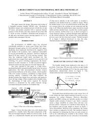
Design of a Hybrid Positioner-Fixture for Six-axis Nanopositioning and Precision FixturingSubmitted to Precision Engineering4.4. System stiffness modelingIn modeling the stiffness of the HPF, we assume that the groove flexure bearing, the guiding flexurebearing and the ball-groove contacts comprise the major sources of compliant deformations. As such,they are modeled as compliant elements, e.g. springs, using the direct stiffness approach. The flexurebearings are modeled as linear compliant elements and the bal-groove joints are modeled as non-linearcompliant Hertzian contacts. Each spring is assigned a local coordinate system. The compliance of theflexible parts (e.g. beams) within each element in the element’s local coordinate system is transformedinto reference frame of the element and the contributions of each flexible part are then combined to forma stiffness matrix for the element. The element’s stiffness characteristics are then transformed into theHPF’s coordinate system and then the contributions of each element are combined to form a stiffnessmatrix for the HPF. This matrix relates the motion of one coupled component (the ball-equippedcomponent) with respect to the grounded (groove-equipped component) under the influence of externalloads. This model was implemented in Matlab and used to predict the system stiffness as a function offixture preload. The change in stiffness with preload (due to the non-linear ball-groove contact stiffness)may be seen in Table 2.Table 2: Simulated HPF stiffness at coupling centroid – based on Matlab modelPreload Kxx[N/µm]Kyy [N/µm] Kzz [N/µm] Kxx[kNm/rad]Kyy[kNm/rad]Kzz[kNm/rad]450N 21.8 21.8 15.5 50.2 50.2 240.8225N 20.4 20.4 14.6 47.3 47.3 223.045N 16.2 16.2 12.1 39.2 39.2 169.85. HPF designThe HPF kinematic and stiffness models were used to design a prototype moving groove HPF. Thecomponents of the prototype are shown in Fig. 16. The structural components and flexures are madefrom 6061 T6 Aluminum. The groove flexures are equipped with a hardened stainless steel plate, called agroove plate, which has been polished to a mirror finish. The plates are bonded to the dorsal surface ofeach groove flexure. The balls are comprised of hardened stainless steel which has been polished tomirror finish. The balls are bonded and pressed into brass collars which are in turn bonded and pressedinto the top octagonal fixture plate. It is this plate which may be used to fixture and position other partswhich are attached to it. The six guide flexures have been cut into a monolithic base component whichis made from 6061 T6 Aluminum.Figure 16: Prototype moving groove HPF, fixture envelope is 250mmx250mmx80mmThe cross section of the ball-grove joint shown in Fig. 17 illustrates how the grooves, groove flexures andgroove plates are rigidly attached to the monolithic base which contains the guiding flexures. Piezoelectricactuators are integrated in the plane of the compliant mechanism such that they are structurally inparallel with their corresponding flexure bearing.14

Design of a Hybrid Positioner-Fixture for Six-axis Nanopositioning and Precision FixturingSubmitted to Precision EngineeringBallCollarPalletClampGrooveplateGroovemountPiezoGrooveflexureBase containingguide flexuresFigure 17: Cross section of a moving groove HPF ball-groove jointFigure 18 provides an exploded view of the HPF in which the assembled relationship between theindividual components is indicated by the parallel dotted lines.Monolithic basePiezo clampGroove flexureBallPalletFigure 18: Exploded view of moving groove HPFGroove platePiezoGroove mountCollarThe models were used to design a HPF with the range characteristics shown in Table 3. The HPF wasdesigned to possess a load capacity of 450 N and motion resolution of 4nm. Stiffness properties will bediscussed in Section 6.6.Table 3: Maximum design range of the moving groove HPF prototypeX[µm]Y[µm]Z[µm]x[µradians]y[µradians]z[µradians]Range ± 25 ± 28 ± 44 ± 480 ± 550 ± 2756. Experiment and discussion of resultsExperiments were run in order to produce data which could be used to (1) ascertain the accuracy of thekinematic model, (2) understand how to calibrate the HPF, (3) verify that the groove flexures preventrelative sliding between the ball and groove, (4) characterize HPF repeatability in fixture mode, (5)ascertain the accuracy of the stiffness modeling and (6) understand the dynamic characteristics of theHPF. The following sub-sections provide summaries of these experiments and discuss the results whichwere obtained.6.1. Experimental setupFigure 19 shows the fixture mounted within an automated test rig. This test rig is equipped with an airpiston which applies up to 450 N nesting preload. A flexure and a wobble pin between the fixture andpiston were used to decouple off-axis preload forces which might be applied by the piston. A dSpacecontrol system, cycles the air piston preload and either acquires readings from six capacitance probes orcontrols the six piezo actuators which position the grooves. High-pressure grease was used at the ball-15

Design of a Hybrid Positioner-Fixture for Six-axis Nanopositioning and Precision FixturingSubmitted to Precision Engineeringgroove interface to reduce settling time of the fixture. The setup was placed on an air table and allowedto come to thermal equilibrium within an insulated enclosure. The uncertainty in the measurement systemvaried for the type of test run, these numbers are reported separately for each test.BaseGrooveflexuresDecouplingflexureFigure 19: Test stand used to characterize HPF performancePalletBall6.2. Positioning: Open-loop performance in a non-calibrated stateDisplacement tests were run to characterize the fixture’s ability to provide pure displacement in each axis.The tests were run prior to calibration and without feedback control. Five positions were measured pertest, one at the home position and two on either side of home. Between each position measurement, thepreload was removed, the grooves were actuated to the desired position and then the preload wasreapplied. The control/data acquisition was programmed to permit the fixture to settle for 30 seconds.Ten readings at each position were taken, and then averaged to obtain the final data point. Theuncertainty of the measurements in this experiment was 60 nm. The displacements and parasitic errorsmeasured in each test are provided in Fig. 20 and Fig. 21. The dotted line in the figures has a slope ofunity and pierces the origin. If no errors are present between commanded and measured displacement, thedata points should lie on this line.16

Design of a Hybrid Positioner-Fixture for Six-axis Nanopositioning and Precision FixturingSubmitted to Precision Engineering50X displacement2X - Parasitic errors20Measured [m]3010-10-30-50-50 -25 0 25 50Command [m]Error [m]10-1-2-50 -25 0 25 50Command [microns]yzTheta xTheta yTheta z100-10-20Error [radian]50Y displacement2Y - Parasitic errors20Measured [m]250-25-50-50 -25 0 25 50Command [m]Error [m]10-1-2xzTheta xTheta yTheta z-50 -25 0 25 50Command [microns]100-10-20Error [radian]50Z displacement2Z - Parasitic errors20Measured [m]250-25-50-50 -25 0 25 50Command [m]Error [m]10-1-2xyTheta xTheta yTheta z-50 -25 0 25 50Command [microns]Figure 20: Translation tests results which compare the measured vs. commanded HPF behavior (left)and the parasitic errors as a function of commanded behavior (right)100-10-20Error [radian]17

Design of a Hybrid Positioner-Fixture for Six-axis Nanopositioning and Precision FixturingSubmitted to Precision EngineeringMeasured [radians]Measured [radians]Measured [radians]5002500-250-500500250x displacement-500 -250 0 250 500Command [radians]0-250-5005002500-250-500y displacement-500 -250 0 250 500Command [radians]z displacement-500 -250 0 250 500Command [radians]Error [m]Error [m]Error [m]1050-5-1010-5-10x - Parasitic errorsxyzTheta yTheta z-500 -250 0 250 500Command [microns]50y - Parasitic errors-500 -250 0 250 500Command [microns]1050-5-10xyzTheta xTheta zz - Parasitic errorsxyzTheta xTheta y-500 -250 0 250 500Command [microns]Figure 21: Orientation tests results which compare the measured vs. commanded HPF behavior (left)and the parasitic errors as a function of commanded behavior (right)Several linear relationships between the commanded displacement and the parasitic errors may bee seenwithin the parasitic error plots. Some of these relationships are denoted on the right sides of Figs. 20 and21 by line fits. The linear relationship between command and error is important as it shows thesesystematic errors are well-correlated to the actuation inputs. This opens the door to an elegant calibrationtechnique which will be described later in this section. The systematic errors are in-part due to:020100-10-202010-10-2020100-10-20Error [radian]Error [radian]Error [radian]18

Design of a Hybrid Positioner-Fixture for Six-axis Nanopositioning and Precision FixturingSubmitted to Precision Engineering(1) Geometry errors: The physical components which define the HPFs kinematic chains differ from theideal components which drive the kinematic model. For example there are errors in the reference andaligning features of each component which affect the assembly of each component. There are also errorsin the size of the components which define the HPFs kinematic chains, repeatable parasitic errors in theguide flexures which are due to imperfect geometry of the compliant parts, and actuator misalignmenterrors.(2) Material property errors: The model assumes isotropic material properties for Aluminum and aYoung’s Modulus of 30 ksi Young’s Modulus. It is not uncommon for the modulus of Aluminum alloyswhich have been formed into sheet to differ by 5-10% fro the generic 30ksi value.6.3. Removing systematic errors via calibrationThe calibrated position and orientation vector, PO C , may be related to the model’s predicted position andorientation vector, PO M , via the calibration matrix, C, given in Eqxn. 29. In this approach, we arecalibrating the HPF by modifying the model rather than modifying the hardware.POCXcYcZc C PO MxcyczcCalibratedC11C21C31C41C51C61C12C22C32C42C52C62C13C23C33C43C53C63C14C24C34C44C54C64C15C25C35C45C55C65C16C26C36C46C56C66XcYcZcxcyczcModelThe rows of the matrix may be populated using the results of the single-axis tests. For instance, during anX axis move, PO M , would be [Xc, 0, 0, 0, 0, 0] T and the pre-calibrated, experimentally determinedposition and orientation vector, PO E , would be given by Eqxn 30.(29)XcYcZcxcycFor POMzcExperimental [ Xc,0,0,0,0,0]TC Xc11C Xc21C Xc31C Xc41C Xc51C Xc61The slope of the lines which were fitted to the data plotted in Figs. 20 and 21 may be used as theconstants, C i1 , for the first column of the calibration matrix. The same procedure may be used to populatethe 2 nd , 3 rd , 4 th , 5 th , and 6 th , columns using the Yc, Zc, xc, yc, and zc tests respectively. Thecompleted matrix for the moving groove HPF prototype is provided in Eqxn. 31.(30)19

Design of a Hybrid Positioner-Fixture for Six-axis Nanopositioning and Precision FixturingSubmitted to Precision Engineering0.9980.013 0.025 0.016 1.000 0.004 0.001 0.007C (31) 0.184 0.950 0.182 1.002 0.016 0.023 0.1740.036 0.0231.0000.6230.110 0.0060.0160.171 0.0310.0010.019 0.003 0.009 0.0200.0011.002 0.0070.0000.003 0.029The improvement due to calibration will depend upon the quality of the line fit. Equation 32 shows theR 2 values for the calibration. The values R ij correspond to the quality of the line fit for C ij .1.0000.7541.0020.614 0.639 1.000 0.929 0.997 0.876R (32)0.705 0.963 0.940 1.000 0.785 0.8350.3180.4510.9861.0000.9940.9500.9660.9980.9830.7980.9531.0000.5780.8581.0000.7841.0000.9190.9940.9930.8621.000The errors in the HPF prototype post calibration are listed in Table 4. The first data set indicates howwell the HPF positions for a commanded single-axis move. The second set looks at the parasitic errorsfor all commanded displacements. In both sets, the numbers in the row labeled “Maximum” are themaximums of the absolute value of the respective error sets.Table 4: HPF positioning errors post calibrationX Y[nm] [nm]Z[nm]x[radian]y[radian]COMMAND DISPLACEMENT1 14 34 26 0.5 0.4 0.2Maximum 36 93 74 1.6 1.0 0.5z[radian]PARASITIC DISPLACEMENTS1 40 50 321 2.2 1.7 0.7Maximum 140 195 1032 7.4 8.8 2.5The parasitic errors are clearly of more concern than the errors in commanded position. In particular, theparasitic errors in the Z axis are significantly larger than those in X and Y. The Z errors are larger as thereis poor correlation between command values and some of the non-calibrated parasitic Z errors. This canbe seen by inspecting the third row of the R matrix. Other parasitic errors (other rows) have several lowR ij values; however the magnitude of the errors for their good (near unity) R ij values is lower than thosefor Z parasitic errors. A direct link between the hardware and the large magnitude/poor correlation of Z20

Design of a Hybrid Positioner-Fixture for Six-axis Nanopositioning and Precision FixturingSubmitted to Precision Engineeringaxis error has not been established. This relationship and other means of reducing parasitic errors are amain focus of continued work.The non-calibrated model links a vector of actuator inputs, A, to the model’s position and orientationvector, PO M , via a transformation matrix, T. The relationship is shown in Eqxn. 33.POM T A(33)PO M is pre-multiplied by the calibration matrix to remove the linear systematic errors from the system.The resulting relationship, shown in Eqxn. 34, links the design parameters of the HPF to the calibratedperformance of the HPF.POC C PO C T A(34)MThe calibrated forward and reverse kinematics may then be calculated via normal matrix multiplicationand inversion techniques. Equation 35 shows the solution for actuation inputs as a function of thecalculated transformation matrix, the calibration and the desired position and orientation. 1 1A T C PO(35)CThe experimental calibration exercise (six tests) takes less than one hour and is therefore a less costly andtime intensive way to achieve better performance in comparison to the setting of tight manufacturing andassembly tolerances. The experimental measurements and subsequent calculations may be automated,thereby making it possible for the HPF to be self calibrating over time.6.4. Verification of no sliding conditionA test was run to determine if the flexures would prevent relative sliding and stick slip at the ball-groovecontacts. For a preload of 225 N, the normal load, F n , on each contact surface is 38-75 N. Thiscorresponds to a tangential contact stiffness of 22 N/µm. The maximum tangential force that may beapplied before slip occurs is given by F t = µ F n , where µ is the static friction coefficient. For lubricatedsteel on steel, µ = 0.16 and the corresponding tangential force, F t , is 12 N. The maximum displacementthat may be expected before siding occurs is 0.5µm. Before the test run, the HPF was engaged, preloadedto 225 N and then allowed to settle for 30 seconds. The HPF was then commanded to move in 4 nmincrements through a range of 3 microns. The results in Fig. 22 do not show discontinuities in the plot.This proves that the groove flexures are successfully preventing relative sliding and stick-slip between theballs and grooves.21

Design of a Hybrid Positioner-Fixture for Six-axis Nanopositioning and Precision FixturingSubmitted to Precision Engineering1500Y displacementCommand [nm ]100050000 500 1000 1500Command [ nm ]Figure 22: Displacement test results for coupling displacement while balls are engaged in groovesAlthough smooth motion of the HPF may be assumed via use of the guiding and groove flexure bearings,it is helpful to validate this behavior and understand the smallest motion increment which may beachieved through the HPF. Figure 23 shows a magnified view of the rectangular detail in Fig. 22. Thefigure indicates that the engaged resolution of the HPF is approximately 4nm. This limit is due tolimitations of the electronics that drive the piezo actuators.Measured [ nm ]250225200175Y displacement (detail)Figure 23: Close up of rectangular detail in Fig. 22150150 175 200 225 250Command [ nm ]6.5. HPF repeatability in fixture modeOne thousand cycles of engagement and disengagement were performed over the course of the 14 hourrepeatability test. The HPF was placed in fixture mode, meaning that the actuators were not used toenhance positioning performance. Positioning occurred solely due to the ball-grove interface interactionsand groove flexure bearing motions. Ideally, the actuators would be commanded to hold their positionthroughout the test. Although the piezos are equipped with internal strain gage sensors which could beused to maintain the position to better than 5nm, the limitations of our dSpace system prevent us fromsimultaneously reading six capacitance probes, reading six strain gages and supplying independentvoltages to the six piezos. A compromise approach was implemented in which the piezo actuators wereenergized with a constant voltage during the duration of the test. As such, the repeatability data willinclude errors from the piezo actuator creep. The results of the test are shown in Fig. 24.22

Design of a Hybrid Positioner-Fixture for Six-axis Nanopositioning and Precision FixturingSubmitted to Precision Engineering2.0X error motion10x error motionX [m]1.00.0-1.0x [radian]50-5-2.00 200 400 600 800 1000Cycle-100 200 400 600 800 1000Cycle2.0Y error motion10y error motionY [m]1.00.0-1.0y [radian]50-5-2.00 200 400 600 800 1000Cycle-100 200 400 600 800 1000Cycle2.0Z error motion10z error motionX [m]1.00.0-1.0z [radian]50-5-2.00 200 400 600 800 1000CycleFigure 24: Repeatability tests with piezo actuators set at constant voltageWe may make several observations from the test results:-100 200 400 600 800 1000Cycle(1) Wear in and long-term stability: Due to the drift – this is clearly seen in the Z data – it is difficult tomake any statements regarding the wear-in behavior of the fixture or the long-term stability. These errorsare not a primary concern as they are known to be on the order of the surface finish [05] and thereforethey may be easily corrected by periodic self-calibration and/or feedback control of the actuators.23

Design of a Hybrid Positioner-Fixture for Six-axis Nanopositioning and Precision FixturingSubmitted to Precision Engineering(2) Random errors: Due to the drift min the piezos, the data should be considered in terms of short-term(point-to-point, PP) performance rather than the long-term (absolute, ABS) performance. Table 5provides the one sigma repeatability in each of the six axes for PP and ABS.Table 5: Fixture repeatability data (values correspond to 1 standard deviation)X[nm]Y[nm]Z[nm]x[radians]y[radians]z[radians]Mates ABS PP ABS PP ABS PP ABS PP ABS PP ABS PP0 - 100 36 14 53 12 68 39 0.60 0.28 0.60 0.28 2.00 0.43700-1000 30 9 34 9 163 35 0.60 0.61 0.60 0.28 2.00 0.270 - 1000 58 11 87 11 288 38 1.4 0.65 1.00 0.29 2.30 0.32The PP values indicate the fixture can be repeatable on the level of tens of nanometers and fractions ofmicro-radians if actuation inputs remain steady. This level of performance from a passive fixture isthought to be due to elimination of ball-groove stick slip. Stick slip prevents the balls from settling intotheir lowest energy state and therefore limits the repeatability of kinematic couplings [11]. As the ballssettle into the grooves, the balls and grooves slide in the directions indicated by the exaggerated wearpatterns in Fig. 8. The groove flexures prevent the random stick slip phenomena at the ball-groovecontacts, thereby enabling the HPF to settle into a state which is closer to its minimum energy state.Although lubricants can be used to reduce this effect [12] when flexure bearings are not used, such anapproach is limited to non-vacuum applications. We hypothesize that the flexures may also reduce thedependence of repeatability on the order of engagement of the balls and grooves. Both issues are subjectsof continued work via experiments on kinematic couplings which are not equipped with actuators, butwhich are equipped with the same groove flexures.6.6. Stiffness characteristicsThe fixture was preloaded to provide approximately 7 N/micron stiffness in the x, y and z directions. TheX and Y stiffness were obtained by hanging weights on the distal end of a string and attaching theproximal end to the fixture. The string was routed such that the tension in the string was directed parallelto the plane of coupling and through the coupling centroid. A comparison of predicted and experimentalresults is provided in Table 6. Experimental results show that the fixture is stiffer than expected byapproximately 30 %. This was expected as the modeling approach assumed conservative values for thestiffness of individual compliant components. A better match between theory and measurement isdesired; therefore future work will be focused upon improving the accuracy of the model.Table 6: HPF stiffness – experimental vs. analytical resultsKx[N/µm]Ky[N/µm]Experimental 10.0 10.0 10.1Analytical model 7.1 7.1 7.3% error 29.7 29.2 27.9Kz[N/µm]24

Design of a Hybrid Positioner-Fixture for Six-axis Nanopositioning and Precision FixturingSubmitted to Precision Engineering6.7. Dynamic characteristicsAlthough the dynamic characteristics of the HPF were not a primary focus of this work, tests wereconducted to compare the behavior of the HPF with dynamic modeling tools which are underdevelopment. The tests were conducted with a preload of 225 N. Figure 25 shows the natural frequencyat 200 Hz for a first mode of translation in the z directions. The majority of the groove-equippedcomponent, e.g. the monolithic base, is physically grounded or directly adjacent to ground during the test,therefore the mass of the top (e.g. ball-equipped component) comprises the major mass which is free tovibrate. It is possible to reduce the mass of this component by 50%, thereby increasing the naturalfrequency up to 40% (280 Hz). If higher frequencies are desired, this can easily be accomplished byincreasing the thickness of the guide flexures and increasing the stiffness of the ball-groove contacts.Norm. response0 100 200 300 400Frequency [ Hz ]Figure 25: Normalized response of HPF dynamic characteristics1.00.507. SummaryIn this paper, we have introduced a hybrid positioning fixture which can be operated in two modes; as (1)a nanometer-level accurate and repeatable exact constraint fixture or (2) as a high load capacity, six-axisnanopositioner. Actuators, sensors and flexures are integrated into the structural loop of the fixture,thereby enabling controlled, changes in fixture geometry to add nanometer/micro-radian-level positioningcapability. The integration of positioning and fixturing functions is made possible by:(a) Ensuring that the flexure bearing’s directions of high compliance are arranged parallel to thedirections in which we wish to actuate. These directions are laid out so that they do not have adetrimental effect on the HPF stiffness when a high-stiffness actuator is used in parallel with the flexure.(b) Ensuring that the flexure bearings’ directions of high stiffness and high load capacity are aligned withthe vectors of force transmittal through the fixture’s structural loop, thereby enabling high load capacityand stiffness.Models of fixture kinematics and fixture stiffness were generated and used to design a proof-of-concept,moving groove HPF prototype. When operated in fixture mode, experiments show standard deviation inpoint-to-point repeatability of 11, 11, and 40nm in x, y, and z; and 0.7, 0.3, and 0.3 micro-radians in x,y and z. When operated in Nanopositioner mode, the device demonstrated 5nm resolution motionincrement and range of 40x40x80 microns in translation and 800x800x400 micro-radians in rotation. Thefixture possesses a load capacity of 450 N, a measured stiffness of 10 N/micron and natural frequency of200 Hz.8. AcknowledgementsThis work was supported, in part, by the Ford Motor Company and the Ford-MIT alliance. The authorswish to thank the alliance and Ford Motor Company for their technical and financial support. Thismaterial is based in-part upon work supported by the National Science Foundation under Grant No.25

Design of a Hybrid Positioner-Fixture for Six-axis Nanopositioning and Precision FixturingSubmitted to Precision Engineering0348242. The authors would also like to thank Mr. Gerry Wentworth and Mr. Mark Belanger for theefforts in fabricating the fixture prototype.9. References[01] Culpepper, M. L., M. K. Varadajan and M. Dibiaso, “Design of integrated eccentric mechanisms and exactconstraint fixtures for micron-level repeatability and accuracy,” Precision Engineering, 29 (1), 65 – 80,January 2005.[02] Barraja, M. and Vallance, R. Tolerance Allocation for Kinematic Couplings, Proceedings of the 2002 ASPESummer Conference, July 2002.[03] Taylor, JB, and Tu, JF Precision X-Y Microstage with maneuverable kinematic coupling mechanism, Prec Eng,April, 1996, vol. 18, No. 2, p.85 – 94.[04] Chui, MA, Roadmap of mechanical systems design for the semiconductor automatic test equipment industry,MIT Ph.D. thesis, 1998.[05] Slocum A. Design of Three-Groove Kinematic Couplings. Prec Eng 1992;14;67-73.[06] Hale, LC., Principles and techniques for designing precision machines, MIT Ph.D. Thesis, 1999, Cambridge,Ma.[07] Schouten CH, Rosielle PCJN, Schellekens PHJ. Design of a kinematic coupling for precision applications. PrecEng;20;46-52.[08] Culpepper, M. L., “Design of Quasi-Kinematic Couplings,” Precision Engineering, 28 (3), 338 – 357, July2004.Mangudi, K. and Culpepper, M. L., “Active, Compliant Fixtures for Nanomanufacturing,” 2004 Annual Meeting ofthe American Society for Precision Engineering, Orlando, FL. October 2004, pp 113 – 116.[09] Culpepper, M. L., A.H. Slocum and F. Z. Shaikh, “Compliant Kinematic Couplings for Use in Manufacturingand Assembly,” Proceedings of the 1998 International Mechanical Engineering Congress and Exposition,Anaheim, CA, November 1998, pp 611 – 8.[10] Mangudi, K. and Culpepper, M. L., “Active, Compliant Fixtures for Nanomanufacturing,” 2004 AnnualMeeting of the American Society for Precision Engineering, Orlando, FL. October 2004, pp 113 – 6.[11] Hale LC, Slocum AH. Optimal Design Techniques for Kinematic Couplings. Prec Eng;25;114-27.[12] Slocum AH, Donmez A. Kinematic couplings for precision fixturing- Part 2: Experimental determination ofrepeatability and stiffness. Prec Eng 1988;10;115-2.26