OCOB Ann Rep 07-08 - Orfalea College of Business - Cal Poly San ...

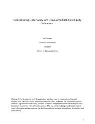
FACULTY REPORTSof losing $100 and a50 percent chanceof winning someamount $Y?” It turnsout that Johnny willshaped value functionhas a kink atthe origin; (iv)while utility iseverywhere concave,turn down anyvalue is con-such bet, no matterhow large Y is. Forexample, Johnnywill turn down a50-50 lose $10/win$2.5 trillion bet! Theonly assumptionsFigure 1: (a) A standard utility function defined over total wealthcave over gains andconvex over losses,i.e., investors arerisk averse whenthey’re winning andrisk-seeking whenthey’re losing – this(asset integration). The concavity of the curve ensures risk aversion.required to reachcaptures two facts:(b) A Kahneman-Tversky style value function defined over losses and gains ratherthis startling conclusionare that Johnnyprefer a sure gain oflaboratory subjectsthan over total wealth. Note (i) the kink at the origin of the value function, and(ii) the red lines indicating the pleasure (pain) caused by unit gain (loss).be an expected utilityThe relatively greater pain caused by unit loss is called “loss aversion.”$100 to the possibilityoptimizer withan increasing andconcave utility-of-wealth function. Rabin and Thaler (ibid.)go on to suggest that “Johnny would, of course, have to beinsane to turn down bets like” these. 1 Suffice it to say thatdecision theorists now regard EUT to be normative in character(how individuals should behave) rather than descriptive(how individuals actually behave).A very considerable effort has gone into formulatingalternatives that capture the systematic patterns whichemerge from field and laboratory experiments in which subjectsare presented with a variety of gambles (lotteries, alsoknown as “prospects”) and asked to choose among them.The weight of evidence suggests that the best candidates fora descriptive theory of choice must have two features: (i)an S-shaped relative value function instead of the monotonicallyincreasing and concave utility-of-wealth function usedin EUT, and (ii) a (subjective) nonlinear transformation ofthe probabilities associated with future outcomes, with verylow probabilities over-weighted (people buy lottery tickets),very high probabilities under-weighted (smokers discountthe risk of falling terribly ill), and mid-range probabilitiesleft unchanged. These “decision weights,” which need notsum to one, are used in place of probabilities when calculatingthe expected “value” of a risky prospect. Figure 1displays a typical EUT-style utility function in panel (a), anda typical behavioral value function in panel (b). Note that(i) utility is defined over total wealth, i.e., the outcomesfrom a gamble are added to pre-gamble wealth before calculatingexpected utility (this is called “asset integration”);(ii) value, however, is calculated without reference to theimpact on a subject’s current or reference wealth; (iii) the S-of winning$200, and that theyprefer the possibility of losing $200 to a sure loss of $100;(v) the slope of the value function over gains in panel 2(b)is less than that of the value function over losses – as thered lines in panel 2(b) indicate, unit loss in wealth causesmore pain than unit gain in wealth causes pleasure, i.e., investorsare loss averse. The combination of decision weightsand an S-shaped value function with the properties outlinedin (ii) through (v) goes a long way in accounting for thechoice behavior exhibited by individuals in real life(Camerer 1992), and avoids anomalies like EUT Johnny’s“insane” behavior.A CAPM-like Model for Loss AversionThe easiest way to obtain a CAPM-like relative pricingmodel for Prospect Theory-style loss averse investors is touse the geometric argument invoked by Sharpe (1964) toget the usual CAPM for mean-variance optimizers. The argumentis illustrated schematically in Figure 2 (see nextpage), using the familiar mean and volatility measures ofreward and risk. The horizontal axis represents the risk ofa portfolio of assets, while the vertical axis represents theassociated reward. The wedge-shaped region represents thefeasible region, i.e., all portfolios that can be constructedfrom available assets with a total investment of zero dollars(this is explained in a bit). A portfolio lying on the upperboundary is said to be efficient (or optimal) because it hasthe lowest risk for a given level of reward. The portfolio Ois one such optimal portfolio. Given an arbitrary portfolioX, we compute its reward (mean excess return over the riskfreerate, or historical risk premium) and its risk (the volatility,or standard deviation, of its historical excess returns)1 Rabin (2000), and Rabin and Thaler (2001) provide a compelling, and entertaining, view of problems that lurk within thestandard EUT paradigm.ORFALEA COLLEGE OF BUSINESS ❚ 15