OCOB Ann Rep 07-08 - Orfalea College of Business - Cal Poly San ...

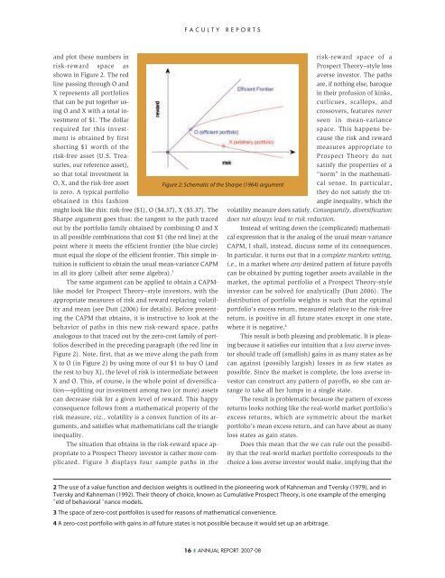
FACULTY REPORTSand plot these numbers inrisk-reward space asshown in Figure 2. The redline passing through O andX represents all portfoliosthat can be put together usingO and X with a total investmentof $1. The dollarrequired for this investmentis obtained by firstshorting $1 worth of therisk-free asset (U.S. Treasuries,our reference asset),so that total investment inO, X, and the risk-free assetis zero. A typical portfolioobtained in this fashionmight look like this: risk-free ($1), O ($4.37), X ($5.37). TheSharpe argument goes thus: the tangent to the path tracedout by the portfolio family obtained by combining O and Xin all possible combinations that cost $1 (the red line) at thepoint where it meets the efficient frontier (the blue circle)must equal the slope of the efficient frontier. This simple intuitionis sufficient to obtain the usual mean-variance CAPMin all its glory (albeit after some algebra). 3The same argument can be applied to obtain a CAPMlikemodel for Prospect Theory–style investors, with theappropriate measures of risk and reward replacing volatilityand mean (see Dutt (2006) for details). Before presentingthe CAPM that obtains, it is instructive to look at thebehavior of paths in this new risk-reward space, pathsanalogous to that traced out by the zero-cost family of portfoliosdescribed in the preceding paragraph (the red line inFigure 2). Note, first, that as we move along the path fromX to O (in Figure 2) by using more of our $1 to buy O (andthe rest to buy X), the level of risk is intermediate betweenX and O. This, of course, is the whole point of diversification—splittingour investment among two (or more) assetscan decrease risk for a given level of reward. This happyconsequence follows from a mathematical property of therisk measure, viz., volatility is a convex function of its arguments,and satisfies what mathematicians call the triangleinequality.The situation that obtains in the risk-reward space appropriateto a Prospect Theory investor is rather more complicated.Figure 3 displays four sample paths in theFigure 2: Schematic of the Sharpe (1964) argumentrisk-reward space of aProspect Theory–style lossaverse investor. The pathsare, if nothing else, baroquein their profusion of kinks,curlicues, scallops, andcrossovers, features neverseen in mean-variancespace. This happens becausethe risk and rewardmeasures appropriate toProspect Theory do notsatisfy the properties of a“norm” in the mathematicalsense. In particular,they do not satisfy the triangleinequality, which thevolatility measure does satisfy. Consequently, diversificationdoes not always lead to risk reduction.Instead of writing down the (complicated) mathematicalexpression that is the analog of the usual mean-varianceCAPM, I shall, instead, discuss some of its consequences.In particular, it turns out that in a complete markets setting,i.e., in a market where any desired pattern of future payoffscan be obtained by putting together assets available in themarket, the optimal portfolio of a Prospect Theory-styleinvestor can be solved for analytically (Dutt 2006). Thedistribution of portfolio weights is such that the optimalportfolio’s excess return, measured relative to the risk-freereturn, is positive in all future states except in one state,where it is negative. 4This result is both pleasing and problematic. It is pleasingbecause it satisfies our intuition that a loss averse investorshould trade off (smallish) gains in as many states as hecan against (possibly largish) losses in as few states aspossible. Since the market is complete, the loss averse investorcan construct any pattern of payoffs, so she can arrangeto take all her lumps in a single state.The result is problematic because the pattern of excessreturns looks nothing like the real-world market portfolio’sexcess returns, which are symmetric about the marketportfolio’s mean excess return, and can have about as manyloss states as gain states.Does this mean that the we can rule out the possibilitythat the real-world market portfolio corresponds to thechoice a loss averse investor would make, implying that the2 The use of a value function and decision weights is outlined in the pioneering work of Kahneman and Tversky (1979), and inTversky and Kahneman (1992). Their theory of choice, known as Cumulative Prospect Theory, is one example of the emerging˚eld of behavioral ˚nance models.3 The space of zero-cost portfolios is used for reasons of mathematical convenience.4 A zero-cost portfolio with gains in all future states is not possible because it would set up an arbitrage.16 ❚ ANNUAL REPORT 2007-08