CashFlow, A Visualization Framework for 3D Flow - Studierstube ...

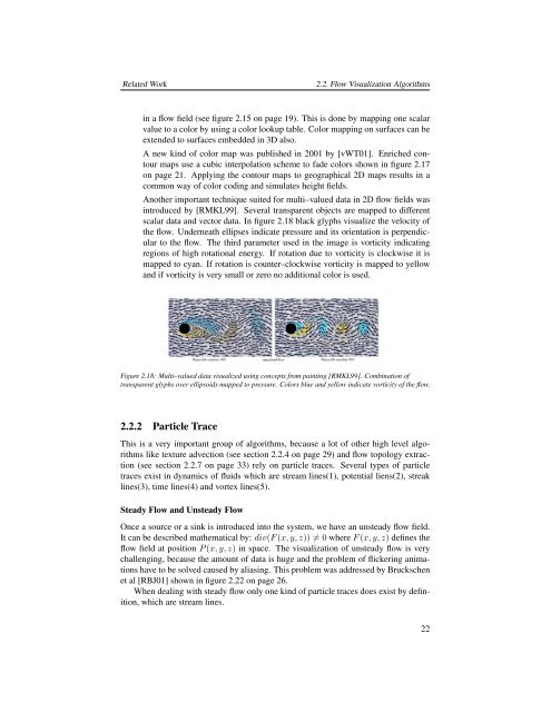
Related Work2.2. Flow Visualization Algorithmsin a flow field (see figure 2.15 on page 19). This is done by mapping one scalarvalue to a color by using a color lookup table. Color mapping on surfaces can beextended to surfaces embedded in 3D also.A new kind of color map was published in 2001 by [vWT01]. Enriched contourmaps use a cubic interpolation scheme to fade colors shown in figure 2.17on page 21. Applying the contour maps to geographical 2D maps results in acommon way of color coding and simulates height fields.Another important technique suited for multi–valued data in 2D flow fields wasintroduced by [RMKL99]. Several transparent objects are mapped to differentscalar data and vector data. In figure 2.18 black glyphs visualize the velocity ofthe flow. Underneath ellipses indicate pressure and its orientation is perpendicularto the flow. The third parameter used in the image is vorticity indicatingregions of high rotational energy. If rotation due to vorticity is clockwise it ismapped to cyan. If rotation is counter–clockwise vorticity is mapped to yellowand if vorticity is very small or zero no additional color is used.Figure 2.18: Multi–valued data visualized using concepts from painting [RMKL99]. Combination oftransparent glyphs over ellipsoids mapped to pressure. Colors blue and yellow indicate vorticity of the flow.2.2.2 Particle TraceThis is a very important group of algorithms, because a lot of other high level algorithmslike texture advection (see section 2.2.4 on page 29) and flow topology extraction(see section 2.2.7 on page 33) rely on particle traces. Several types of particletraces exist in dynamics of fluids which are stream lines(1), potential liens(2), streaklines(3), time lines(4) and vortex lines(5).Steady Flow and Unsteady FlowOnce a source or a sink is introduced into the system, we have an unsteady flow field.It can be described mathematical by: div(F (x, y, z)) ≠ 0 where F (x, y, z) defines theflow field at position P (x, y, z) in space. The visualization of unsteady flow is verychallenging, because the amount of data is huge and the problem of flickering animationshave to be solved caused by aliasing. This problem was addressed by Bruckschenet al [RBJ01] shown in figure 2.22 on page 26.When dealing with steady flow only one kind of particle traces does exist by definition,which are stream lines.22