- Page 6: Jochen KämpfAdvanced Ocean Modelli
- Page 12: viPrefaceconvection model, a proble
- Page 18: Contentsix3.7.3 Theory . . ........
- Page 24: xiiContents4.6 Exercise19:EkmanPump
- Page 28: Chapter 1IntroductionAbstract This
- Page 32: 1.1 Fundamental Physical Laws 3When
- Page 36: 1.3 Modelling with FORTRAN 95 5∂
- Page 40: 1.4 Visualisation with SciLab 7http
- Page 46: 10 2 1D Models of Ekman LayersFig.
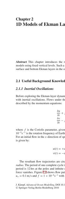
- Page 50: 12 2 1D Models of Ekman Layersthe o
- Page 54: 14 2 1D Models of Ekman LayersUse o
- Page 58: 16 2 1D Models of Ekman Layerswhere
- Page 62: 18 2 1D Models of Ekman Layers2.4 T
- Page 66: Chapter 3Basics of Nonhydrostatic M
- Page 70: 3.2 2D Vertical-Slice Modelling 23F
- Page 74: 3.3 Surface Gravity Waves 25where
- Page 78: 3.4 Nonhydrostatic Solver 27imposed
- Page 82: 3.4 Nonhydrostatic Solver 29Fig. 3.
- Page 86: 3.4 Nonhydrostatic Solver 31Fig. 3.
- Page 90: 3.5 Exercise 3: Short Surface Gravi
- Page 94:
3.6 Inclusion of Variable Density 3
- Page 98:
3.6 Inclusion of Variable Density 3
- Page 102:
3.6 Inclusion of Variable Density 3
- Page 106:
3.7 Exercise 4: Density-Driven Flow
- Page 110:
3.7 Exercise 4: Density-Driven Flow
- Page 114:
3.8 Internal Waves 45which implies
- Page 118:
3.9 Exercise 5: Internal Waves 47Fi
- Page 122:
3.10 Mechanical Turbulence 49Fig. 3
- Page 126:
3.11 Exercise 6: Kelvin-Helmholtz I
- Page 130:
3.12 Lee Waves and the Froude Numbe
- Page 134:
3.13 Exercise 7: Lee Waves 55case s
- Page 138:
3.14 Oceanic Convection 57Further e
- Page 142:
3.14 Oceanic Convection 59Considera
- Page 146:
3.15 Exercise 8: Free Convection 61
- Page 150:
3.15 Exercise 8: Free Convection 63
- Page 154:
3.16 Exercise 9: Convective Entrain
- Page 158:
3.17 Exercise 10: Slope Convection
- Page 162:
3.17 Exercise 10: Slope Convection
- Page 166:
3.17 Exercise 10: Slope Convection
- Page 170:
3.18 Double Diffusion 733.18.3 Doub
- Page 174:
3.19 Exercise 11: Double-Diffusive
- Page 178:
3.20 Exercise 12: Double-Diffusive
- Page 182:
3.21 Tilted Coordinate Systems 79Fi
- Page 186:
3.22 Exercise 13: Stratified Flows
- Page 190:
3.23 Estuaries 83The dynamic instab
- Page 194:
3.23 Estuaries 85instance of maximu
- Page 198:
3.23 Estuaries 87found underneath t
- Page 202:
3.24 Exercise 14: Positive Estuarie
- Page 206:
3.24 Exercise 14: Positive Estuarie
- Page 210:
3.24 Exercise 14: Positive Estuarie
- Page 214:
3.25 Exercise 15: Inverse Estuaries
- Page 218:
Chapter 42.5D Vertical Slice Modell
- Page 222:
4.1 The Basis 99to the centre of th
- Page 226:
4.1 The Basis 101The speed of front
- Page 230:
4.2 Exercise 16: Geostrophic Adjust
- Page 234:
4.2 Exercise 16: Geostrophic Adjust
- Page 238:
4.3 Exercise 17: Tidal-Mixing Front
- Page 242:
4.3 Exercise 17: Tidal-Mixing Front
- Page 246:
4.4 Coastal Upwelling 1114.4.2 How
- Page 250:
4.5 Exercise 18: Coastal Upwelling
- Page 254:
4.5 Exercise 18: Coastal Upwelling
- Page 258:
4.5 Exercise 18: Coastal Upwelling
- Page 262:
4.6 Exercise 19: Ekman Pumping 119i
- Page 266:
4.6 Exercise 19: Ekman Pumping 121w
- Page 270:
4.6 Exercise 19: Ekman Pumping 123F
- Page 274:
Chapter 53D Level ModellingAbstract
- Page 278:
5.2 Numerical Treatment 127Vertical
- Page 282:
5.2 Numerical Treatment 129Fig. 5.2
- Page 286:
5.3 Exercise 20: Geostrophic Adjust
- Page 290:
5.4 Exercise 21: Eddy Formation in
- Page 294:
5.4 Exercise 21: Eddy Formation in
- Page 298:
5.5 Exercise 22: Exchange Flow Thro
- Page 302:
5.5 Exercise 22: Exchange Flow Thro
- Page 306:
5.5 Exercise 22: Exchange Flow Thro
- Page 310:
5.6 Exercise 23: Coastal Upwelling
- Page 314:
5.6 Exercise 23: Coastal Upwelling
- Page 318:
5.7 The Thermohaline Circulation 14
- Page 322:
5.8 Exercise 24: The Abyssal Circul
- Page 326:
5.8 Exercise 24: The Abyssal Circul
- Page 330:
5.8 Exercise 24: The Abyssal Circul
- Page 334:
5.9 The Equatorial Barrier 155first
- Page 338:
5.9 The Equatorial Barrier 157Fig.
- Page 342:
5.10 Equatorial Waves 159The soluti
- Page 346:
5.11 The El-Niño Southern Oscillat
- Page 350:
5.12 Exercise 25: Simulation of an
- Page 354:
5.12 Exercise 25: Simulation of an
- Page 358:
5.13 Advanced Lateral Boundary Cond
- Page 362:
5.13 Advanced Lateral Boundary Cond
- Page 366:
5.15 Technical Information 1715.14
- Page 370:
174 BibliographyHelmholtz, H. L. F.
- Page 376:
List of Exercises2.3 Exercise 1: Th
- Page 382:
180 IndexCorilios parameter, 2, 9,