Porosity Aware Buffered Steiner Tree Construction - Computer ...

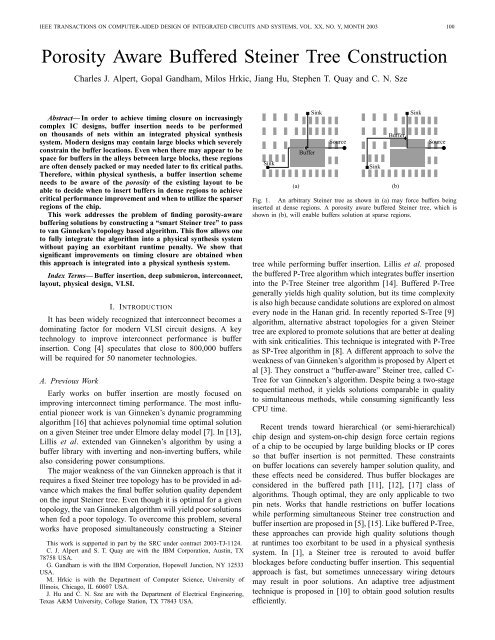
IEEE TRANSACTIONS ON COMPUTER-AIDED DESIGN OF INTEGRATED CIRCUITS AND SYSTEMS, VOL. XX, NO. Y, MONTH 2003 100Porosity Aware Buffered Steiner Tree ConstructionCharles J. Alpert, Gopal Gandham, Milos Hrkic, Jiang Hu, Stephen T. Quay and C. N. SzeAbstract— In order to achieve timing closure on increasinglycomplex IC designs, buffer insertion needs to be performedon thousands of nets within an integrated physical synthesissystem. Modern designs may contain large blocks which severelyconstrain the buffer locations. Even when there may appear to bespace for buffers in the alleys between large blocks, these regionsare often densely packed or may needed later to fix critical paths.Therefore, within physical synthesis, a buffer insertion schemeneeds to be aware of the porosity of the existing layout to beable to decide when to insert buffers in dense regions to achievecritical performance improvement and when to utilize the sparserregions of the chip.This work addresses the problem of finding porosity-awarebuffering solutions by constructing a “smart Steiner tree” to passto van Ginneken’s topology based algorithm. This flow allows oneto fully integrate the algorithm into a physical synthesis systemwithout paying an exorbitant runtime penalty. We show thatsignificant improvements on timing closure are obtained whenthis approach is integrated into a physical synthesis system.Index Terms— Buffer insertion, deep submicron, interconnect,layout, physical design, VLSI.I. INTRODUCTIONIt has been widely recognized that interconnect becomes adominating factor for modern VLSI circuit designs. A keytechnology to improve interconnect performance is bufferinsertion. Cong [4] speculates that close to 800,000 bufferswill be required for 50 nanometer technologies.A. Previous WorkEarly works on buffer insertion are mostly focused onimproving interconnect timing performance. The most influentialpioneer work is van Ginneken’s dynamic programmingalgorithm [16] that achieves polynomial time optimal solutionon a given Steiner tree under Elmore delay model [7]. In [13],Lillis et al. extended van Ginneken’s algorithm by using abuffer library with inverting and non-inverting buffers, whilealso considering power consumptions.The major weakness of the van Ginneken approach is that itrequires a fixed Steiner tree topology has to be provided in advancewhich makes the final buffer solution quality dependenton the input Steiner tree. Even though it is optimal for a giventopology, the van Ginneken algorithm will yield poor solutionswhen fed a poor topology. To overcome this problem, severalworks have proposed simultaneously constructing a SteinerThis work is supported in part by the SRC under contract 2003-TJ-1124.C. J. Alpert and S. T. Quay are with the IBM Corporation, Austin, TX78758 USA.G. Gandham is with the IBM Corporation, Hopewell Junction, NY 12533USA.M. Hrkic is with the Department of Computer Science, University ofIllinois, Chicago, IL 60607 USA.J. Hu and C. N. Sze are with the Department of Electrical Engineering,Texas A&M University, College Station, TX 77843 USA.Sink(a)BufferSinkSourceSinkBuffer(b)SinkSourceFig. 1. An arbitrary Steiner tree as shown in (a) may force buffers beinginserted at dense regions. A porosity aware buffered Steiner tree, which isshown in (b), will enable buffers solution at sparse regions.tree while performing buffer insertion. Lillis et al. proposedthe buffered P-Tree algorithm which integrates buffer insertioninto the P-Tree Steiner tree algorithm [14]. Buffered P-Treegenerally yields high quality solution, but its time complexityis also high because candidate solutions are explored on almostevery node in the Hanan grid. In recently reported S-Tree [9]algorithm, alternative abstract topologies for a given Steinertree are explored to promote solutions that are better at dealingwith sink criticalities. This technique is integrated with P-Treeas SP-Tree algorithm in [8]. A different approach to solve theweakness of van Ginneken’s algorithm is proposed by Alpert etal [3]. They construct a “buffer-aware” Steiner tree, called C-Tree for van Ginneken’s algorithm. Despite being a two-stagesequential method, it yields solutions comparable in qualityto simultaneous methods, while consuming significantly lessCPU time.Recent trends toward hierarchical (or semi-hierarchical)chip design and system-on-chip design force certain regionsof a chip to be occupied by large building blocks or IP coresso that buffer insertion is not permitted. These constraintson buffer locations can severely hamper solution quality, andthese effects need be considered. Thus buffer blockages areconsidered in the buffered path [11], [12], [17] class ofalgorithms. Though optimal, they are only applicable to twopin nets. Works that handle restrictions on buffer locationswhile performing simultaneous Steiner tree construction andbuffer insertion are proposed in [5], [15]. Like buffered P-Tree,these approaches can provide high quality solutions thoughat runtimes too exorbitant to be used in a physical synthesissystem. In [1], a Steiner tree is rerouted to avoid bufferblockages before conducting buffer insertion. This sequentialapproach is fast, but sometimes unnecessary wiring detoursmay result in poor solutions. An adaptive tree adjustmenttechnique is proposed in [10] to obtain good solution resultsefficiently.

IEEE TRANSACTIONS ON COMPUTER-AIDED DESIGN OF INTEGRATED CIRCUITS AND SYSTEMS, VOL. XX, NO. Y, MONTH 2003 101000000000111111111000000000111111111000000000111111111000000000111111111000000000111111111Sink000000000011111111110000000000111111111100000000001111111111000000000011111111110000000000111111111100000000001111111111000000000011111111110000000000111111111100000000001111111111Buffer(a)SinkSource00000000111111110000000011111111000000001111111100000000111111110000000011111111SinkSink000000000001111111111100000000000111111111110000000000011111111111000000000001111111111100000000000111111111110000000000011111111111000000000001111111111100000000000111111111110000000000011111111111Buffer(b)SourceFig. 2. An arbitrary Steiner tree as shown in (a) may force wires to passthrough routing congested regions. A congestion aware buffered Steiner tree,which is shown in (b), will may let wires go through sparse regions.B. The Importance of PorosityIn tradition design flows, buffer insertion is applied afterplacement to optimize interconnect timing. As interconnecteffects become increasingly severe, buffer insertion needs to bepushed up earlier in the design flow to help logic optimizationand placement algorithms on interconnect estimation and toreserve buffering resources. The sheer number of nets thatrequire buffering means that resources need to be allocatedintelligently. For example, large blocks placed close togethercreate narrow alleys that are magnets for buffers since theyare the only locations that buffers can be inserted for routesthat cross over these blocks. But competition for resources forthese routes is very fierce. Inserting buffers for less criticalnets can eliminate space that is needed for more critical netsthat may require gate sizing or other logic transforms. Further,though no blockages lie in the alleys, these regions couldalready be packed with logic and no feasible space for thebuffer might exist. If the buffer insertion algorithm cannotrecognize this scenario then inserting a buffer into this spacemay cause placement legalization to spiral it out to a regiontoo far from its original location. Hence, whenever possibleone should avoid denser regions unless absolutely critical.For example, Figure 1(a) shows a net which is routedthrough a dense region or “hot spot”, and Figure 1(b) showsthe net routed differently to avoid this congested region.In addition to porosity (or placement congestion), a buffersolution may generate remarkable impact on wiring congestionas well. Figure 2 (a) and (b) show an example for a multi-pinnet where the Steiner point needs to be moved outside of thedense region to yield less wiring congestion.The literature contains no buffering approach which addressesthese issues. Note that several algorithms (such asS-Tree and SP-Tree) could be used to address porosity constraintssince they can be run on arbitrary grid graphs. However,the extensions are hardly straightforward. One has tocarefully consider the weighting scheme for edges in the gridgraph, how to sparsify the graph to give reasonable runtimes,the appropriate cost functions, etc. Further, any simultaneousapproach is likely to require too much runtime to be practicallyused within physical synthesis.This work proposes a porosity aware buffered Steiner treeconstruction and is the first buffer insertion work to addressporosity in the layout directly (as opposed to simply specifyinga handful of allowable buffer insertion locations). Theapproach begins with a timing-driven but porosity-ignorantSteiner tree, then applies a plate-based adjustment guidedby length based buffer insertion. After performing localizedblockage avoidance, the resulting tree is then passed to vanGinneken’s algorithm to obtain a porosity aware bufferedSteiner tree. Physical synthesis experiments on real industrialcircuits confirms the effectiveness of this framework.II. PROBLEM FORMULATIONThe porosity is represented through a tile graph G(V G ,E G )where a node g ∈ V G corresponds to a tile and an edge e uv ∈E G represents a boundary between two neighboring tiles uand v ∈ V G . A high porosity implies a low congestion ordensity, vice versa. If a tile g ∈ V G has an area of A(g)and its area occupied by placed cells are a(g), the placementdensity is defined as the area usage density d(g) = a(g)A(g)oftile g. For the boundary between two adjacent tiles g i andg j , its wire density d(g i ,g j ) is the number of wires across itdivided by the number of wiring tracks across this boundary.We take d 2 (g i ,g j ) as wire density cost in our implementation.We address the following problem:Porosity-aware Buffered Steiner Tree Problem: Givena net N = {v 0 ,v 1 ,...,v n } with source v 0 and sinks{v 1 ,...,v n }, load capacitance c(v i ) and required arrival timeq(v i ) for 1 ≤ i ≤ n, tile graph G(V G ,E G ), and a buffer type b,construct a Steiner tree T (V,E), in which V = N ∪ V Steinerand edges in E span every node in V , such that a bufferinsertion solution that satisfies q(v i ) may be obtained with aminimal porosity cost(wire density cost).For porosity cost, one can sum the costs of the tiles that theroutes cross. We use the following function, though certainlyothers can be used as well, depending on the application. Foreach buffer inserted in a tile g, the porosity cost p(g) is definedas:⎧⎨0.5 : d(g) ≤ 0.5p(g) = 4d 2 (g) − 2d(g)+0.5 : 0.5

IEEE TRANSACTIONS ON COMPUTER-AIDED DESIGN OF INTEGRATED CIRCUITS AND SYSTEMS, VOL. XX, NO. Y, MONTH 2003 102SourceSourcev1v5v1v5v1v5v4v3v4v3v4v3v2v2v2(a)(b)(c)Fig. 3. (a) Candidate solutions are generated from v 2 and v 3 and propagated to every tile, which is shaded, in the plate for v 4 . Solution search is limitedto the bounding boxes indicated by the thickened dashed lines. (b) Solutions from v 1 and every tile in the plate for v 4 are propagated to the plate for v 5 . (c)Solutions from plate of v 5 are propagated to the source and the thin solid lines indicate an alternative tree that may result from this process.a van Ginneken style buffer insertion algorithm that employshigher order delay models, handles slew and load capacitanceconstraints, manages a library of inverting and non-invertingbuffers and trades off buffer resource utilization with solutionquality. Integrating a Steiner tree construction into this algorithmwhile maintaining all its features would be prohibitive.However, just constructing a Steiner tree without performingbuffer insertions cannot possibly yield the best topology.Therefore, we propose to solve the porosity aware bufferedSteiner tree problem through the following four stages:1) Initial porosity ignorant timing-driven Steiner tree construction2) Plate-based adjustment for porosity improvement3) Local blockage avoidance4) Van Ginneken style buffer insertionFor stage one, one can construct a timing-driven Steiner treethrough any heuristics. We choose to apply the “buffer aware”C-Tree algorithm [3]. The C-Tree algorithm first clusters thesinks according to their timing criticality, signal polarity andlocation proximity. Then a timing driven Steiner tree algorithmis applied to obtain the intra-cluster and inter-cluster routings.Stage 2 contains the key ideas behind the algorithm. Theplate-based adjustment phase modifies the existing timingdrivenSteiner in an effort to reduce congestion cost whilemaintaining the tree’s high performance. One of the key elementsis that it allows Steiner points to migrate outside of highporositytiles into lower-porosity tiles to reduce congestionwhile maintaining (if not improving) performance.After Stage 2, the Steiner tree is correct in that it goesthrough the tiles that optimize performance while minimizingporosity cost, though the routes may overlap blockages. Performinglocal blockage avoidance in Stage 3, manipulates theroutes within each tile to avoid blockages, thereby allowingmore buffer insertion candidates. However, this stage does notdisturb the tree topology uncovered from Stage 2.Finally, in Stage 4 the resulting tree topology is fixed for vanGinneken style buffer insertion [16]. Van Ginneken’s algorithmis a dynamic programming based bottom-up approach. A setof candidate solutions are propagated from leaf nodes towardthe source and the optimal solution is selected at the source.Since we use known algorithms for Stages 1 and 4, the restof the discussion focuses on the other two stages.B. Stage 2: Plate-based AdjustmentsThe basic idea for the plate-based adjustment is to perform asimplified simultaneous buffer insertion and local tree adjustmentso that the Steiner nodes and wiring paths can be movedto regions with greater porosity without significant disturbanceon the timing performance obtained in Stage 1.The buffer insertion scheme employed here is similar to thelength based buffer insertion in [2]. However, we allow theSteiner points and wiring paths to be adjusted. This approachis also distinctive from a simultaneous buffer insertion andSteiner tree construction approach [14] in which the Steinertree is built from scratch. The plate-based adjustment traversesthe given Steiner topology in a bottom-up fashion similar tovan Ginneken’s algorithm. During this process, Steiner nodesand wiring paths may be adjusted together with buffer insertionto generate multiple candidate solutions.The range of the moves are restrained by the plates definedas follows. For a node v i ∈ T (V,E) which is located in a tileg k ,aplate P (v i ) for v i is a set of tiles in the neighborhood ofg k including g k itself. During the plate-based adjustment, weconfine the location change for each Steiner node within itscorresponding plate. If v i is a sink or the source node we letP (v i )={g k }. For example, when v i is a branch node, we setP (v i ) to be the 3 × 3 array of tiles centered at g k . Of course,if g k lies on the border of the entire tile graph, P (v i ) mayinclude fewer tiles. Figure 3(a) gives an example of the platecorresponding to Steiner node v 4 . The plate indicates any ofthe possible location which the Steiner node may be movedto. This example shows the Steiner node being moved up onetile and right one tile.The search for alternate wiring paths is limited to theminimum bounding box covering the plates of two endnodes. In Figure 3, such bounding boxes are indicated by thethickened dashed lines. Therefore, the size of plates definethe search range for both Steiner nodes and wiring paths.

IEEE TRANSACTIONS ON COMPUTER-AIDED DESIGN OF INTEGRATED CIRCUITS AND SYSTEMS, VOL. XX, NO. Y, MONTH 2003 103Certainly, a plate may be defined to include more tiles orto even be a irregular shape. For example, if the plate sizeis 1 × 1, our algorithm will basically reduce to a lengthbased/van Ginneken style buffer insertion algorithm along afixed topology. However, one could also choose the plate tobe the entire tile graph – this yields an algorithm similar tothe S-Tree embedding [9]. By choosing a plate of size largerthan one but smaller than the entire grid graph, we still obtainthe ability to modify the topology to move critical Steinerpoints into low-porosity regions while also capping the runtimepenalty. Hence, our experiments use a 3×3 tile size to capturethis tradeoff. An example of how a new Steiner topology mightbe constructed from an existing topology is demonstrated inFigures 3(a)-(c).Adopting a length-based buffer insertion scheme [2] makesthe adjustment simpler and thereby faster. Since this stageonly produces a Steiner tree before buffering, the purpose ofincluding buffering at this stage is for estimation purposes,hence a simplified scheme should be adequate.Alpert et al. [2] suggest that buffer insertion may beperformed in a simple way by just following a rule of thumb:the maximal interval between two neighboring buffers isno greater than certain upper bound. The interval betweenneighboring buffers is specified in term of number of tiles. Inthis work, this constraint is modified to be the maximum loadcapacitance U a buffer/driver may drive, so that sink/buffercapacitance can be incorporated. To keep the succinctness ofthe tile-based interval metric in [2], we discretize the loadcapacitance in units equivalent to the capacitance of wirewith average tile size. If the average tile boundary lengthis λ and the wire capacitance per unit length is ĉ, then aload capacitance is expressed in the number of θ = λĉ. Thismodification allows us to use non-uniform sized tiles, eventhough we still assume such non-uniformity is very limited.Fig. 4.Procedure: F indCandidates(v)Input: Current node v to be processedOutput: Candidate solution set S(P (v))Global: Steiner tree T (V,E)Tile graph G(V G ,E G )1. If v is a sinkS(v) ←{(v, 0, 0)}S(P (v)) ←{S(v)}Return S(P (v))2. v l ← left child of vS(P (v l )) ← F indCandidates(v l )3. S l (P (v)) ← P ropagate(S(P (v l )),P(v))4. If v has only one childReturn S l (P (v))5. v r ← right child of vS(P (v r )) ← F indCandidates(v r )6. S r (P (v)) ← P ropagate(S(P (v r )),P(v))7. S(P (v)) ← Merge(S l (P (v)),S r (P (v))8. Return S(P (v))Core algorithm.Also for the sake of simplification, we assume a single“typical” buffer type, the Elmore delay model for interconnectand a switch level RC gate delay model for this plate-basedadjustment.Each intermediate buffer solution is characterized by a 3-tuple s(v, c, w) in which v is the root of the subtree, c isthe discretized load capacitance seen from v, and w is theaccumulated porosity cost. A solution s i (v, c i ,w i ) is said tobe dominated by another solution s j (v, c j ,w j ),ifc i ≥ c j andw i ≥ w j . A set of buffer solutions S(v) at node v is a nondominatingset when there is no solution in S(v) dominated byanother solution in S(v). Usually S(v) is arranged as an array{s 1 (v, c 1 ,w 1 ),s 2 (v, c 2 ,w 2 )...} in the ascending order of loadcapacitance. The basic operations of the length-based bufferinsertion are:Procedure: P ropagate(S(P (v i )),P(v j ))Input: Candidate solutions at P (v i )Expansion region P (v j )Output: Candidate solution set S(P (v j ))0. S(P (v j )) ←∅B ← bounding box of P (v i ) and P (v j )Q ←∅1. For each tile g k ∈ P (v i )Q ← Q ∪ S(g k )2. While Q ≠ ∅3. s ← min cost solution in Qg k ← tile where s locates4. For each tile g l adjacent to g k5. If g l ∈ BExpand(s(g k ),g l )Prune Q6. Return S(P (v j ))Fig. 5. Subroutine of propagating candidate solutions from one plate toanother plate.• AddW ire(s i (v, c i ,w i ),u): grow solution s i at v to nodeu by adding a shortest distance wire between them. Nodeu is either within the same tile as v or in the neighboringtile of v. If the wire has capacitance C, we can getc j (u) =c i (v)+ C θand w j(u) =w i (v)+γl(v, u) wherel(v, u) is the rectilinear distance between v and u dividedby the average tile size and γ is a weighting factor. Sincethe expansion step is one tile, l(v, u) is normally a valuearound 1. When the wiring congestion is considered, wewill count the wire density d(u, v) which is the ratio ofthe number of wires across the boundary between u and vto the number of wiring tracks there. Thus, an additionalterm βd 2 (u, v) is added to w j (u). The coefficient β is anweighting factor.• AddBuffer(s i (v, c i ,w i )): insert buffer at v. If bufferb has an input capacitance c b , output resistance r b andintrinsic delay t b , then the buffered solution s j (v, c j ,w j )is characterized by c j (v) =c b /θ and w j (v) =w i (v) +αp(g) in which p(g) is the porosity cost defined inSection II and α is its weighting factor.• Prune(S(v)): remove any solution s i ∈ S(v) that isdominated by another solution s j ∈ S(v).

IEEE TRANSACTIONS ON COMPUTER-AIDED DESIGN OF INTEGRATED CIRCUITS AND SYSTEMS, VOL. XX, NO. Y, MONTH 2003 104to be removed from Q as well. When the candidate solutionexpansion reaches node v j , solution set S(P (v j )) is updated.(a)(c)Fig. 6. A path overlaps with a buffer blockage as in (a) can be moved outof the blockage with a small detour as in (b) with a small penalty coefficienton cost. Only a greater penalty coefficient can allow a large detour like from(c) to (d).• Expand(s i (v, c i ,w i ),u): grow s i (v) to node u byAddW ire to get solution s j (u, c j ,w j ), insert bufferfor s j (u) to obtain s k (u, c k ,w k ). Add the unbufferedsolution s j and buffered solution s k into solution set S(u)and prune the solutions in S(u).• Merge(S l (v),S r (v)): merge solution set from left childof v to the solution set from the right child of v to obtain amerged solution set S(v). For a solution s i,l (v, c i,l ,w i,l )from the left child and a solution s j,r (v, c j,r ,w j,r ), theyare merged to s k (v, c k = c i,l + c j,r ,w k = w i,l + w j,r )only when c k ≤ U.Similar to the van Ginneken’s algorithm, starting from theleaf nodes, candidate solutions are generated and propagatedtoward the source in a bottom-up manner. Before we propagatecandidate solutions from node v i to its parent node v j ,wefirstfind both plate P (v i ) and plate P (v j ) and define a boundingbox which is the minimum sized array of tiles covering bothP (v i ) and P (v j ). Then we propagate all the candidate solutionsfrom each tile of P (v i ) to each tile of P (v j ) within thisbounding box. Note that branch nodes are allowed to be movedin a neighborhood defined by the plate. Since the branchnodes are more likely to be buffer sites due to the demandon decoupling non-critical branch load from the critical path,allowing branch nodes to be moved to less congested areais especially important. Moreover, such move is a part of acandidate solution, thus such move will be committed onlywhen its corresponding candidate solution is finally selected atthe driver. Therefore, such move is dynamically generated andselected according to the request of the final minimal porositycost solution. The generality of this adjustment algorithmallows its application on alleviating wiring congestion simplythrough incorporating a cost reflecting the wire density inAddW ire().The complete description on the core algorithm is givenin Figure 4 and the subroutine of solution propagation is inFigure 5. In the process of candidate solution propagation(Figure 5), a priority queue Q is employed to maintain thewavefront solutions. In line 5 of Figure 5, if a solution atg l is in Q and is pruned out in Expand(s(g k ),g l ), it needs(b)(d)C. Stage 3: Local Blockage AvoidanceAfter the tree has been modified to route through the tileswith high porosity, the tree still may overlap blockages. Thisis especially true if one uses a sparse grid graph to beginwith. This occurs because the plate-based adjustment in Stage2 is performed with respect to a given tile graph, but largeblockages themselves are managed as part of a tile. Forexample, if a blockage occupies half the area of a given tile,but the remaining half of the tile is empty, the tile’s density is50%. Of course, a net that traverses through this tile shouldbe routed in the space not occupied by the blockage whereverpossible. Thus, this stage performs local cleanup within tiles toachieve blockage avoidance without changing tile assignment.The local blockage avoidance is similar to the algorithmproposed in [1]. The main idea is to divide each Steiner treeinto a set of non-overlapping 2-paths and then perform localblockage avoidance on each 2-path. A 2-path is a path of nodesfor a given Steiner tree such that both endpoints are either thesource, a sink, or a Steiner node with degree greater than two.Each 2-path of a given Steiner tree is rerouted over anextended Hanan grid generated by drawing horizontal andvertical lines through each pin and extending the borders ofeach rectangle shaped buffer blockage. The extended Hanangrids are shown by the dashed lines in Figure 6. In this grid,if an edge does not overlap with any blockage, its cost isits geometric length. Otherwise, edge cost will be geometriclength timed by a penalty coefficient greater than one. Aminimal cost path is searched over this grid to replace original2-path to achieve blockage avoidance. The value of the penaltycoefficient controls the tradeoff between blockage avoidanceand total wirelength. A greater value of the penalty coefficientimplies a stronger desire to avoid the blockage and a greaterwiring detour is allowed. A small penalty coefficient willrestrict the total wirelength with a reduced blockage avoidanceability. Such tradeoff is illustrated in Figure 6.During seeking the minimal cost path in [1], the entireregion covering the two endpoints are expanded properly andare searched. For the example in Figure 7(a), when the 2-pathbetween v 3 and v 5 is rerouted, the search region is indicated bythe thickened dashed lines in Figure 7(a). In our case, since theSteiner tree after stage 2 is already in high porosity regions, wemay refine the search region to be the tiles the 2-path passingthrough as shown by the thickened dashed lines in Figure 7(b).In this work, we define the penalty coefficient to be 1.01 sothat the wire detour from this rerouting will be very small (nomore than 1% wirelength increase) and the disturbance to thetiming performance of the tree is very limited. In Figure 7,the rerouted path after blockage avoidance is shown in (b).IV. EXPERIMENTAL RESULTSIn order to test the effectiveness of our algorithm, weperform experiments in three scenarios: (1) experiments onseveral large nets to observe the effect on porosity; (2) experimentswith consideration on wiring congestion; (3) applying

IEEE TRANSACTIONS ON COMPUTER-AIDED DESIGN OF INTEGRATED CIRCUITS AND SYSTEMS, VOL. XX, NO. Y, MONTH 2003 105SourceSourcev4v1v4v1v5v2v5v2v3v3(a)(b)Fig. 7. An example of local blockage avoidance. Shaded rectangles represent buffer blockages. The Steiner tree before blockage avoidance (a) and afterblockage avoidance (b).our algorithm into an industrial design flow to evaluate impacton overall circuit timing performance.A. Experiments Considering Porosity76stages 1−4stages 1−3−4stages 1−2−3−4TABLE IBENCHMARK CIRCUITS.THE SLACK UNIT IS ps.Net # sinks Max slack Min slack Grid sizemcu0s5 18 6596.0 6195.3 29 × 31mcu1s9 19 6507.3 6247.7 40 × 30n1071 17 2560.4 1902.4 26 × 42n18905 29 6650.3 609.5 58 × 46n313 19 6704.4 1232.5 52 × 65n7866 32 6703.5 96.9 88 × 36n8692 21 6390.1 1053.9 74 × 26n8702 43 6588.5 739.3 64 × 41n8730 20 6656.2 729.5 58 × 35netbig1 88 159564.7 1974 65 × 90netbig2 79 65837.9 104.2 47 × 31netbig3 63 40643.2 1327.4 42 × 36Total porosity cost54321100 150 200 250 300 350 400 450Slack improvement/psFig. 8.The cost-slack trade-off curves for net mcu0s5.The statistics for the benchmark circuits are shown inTable I. These nets are extracted from industrial circuits withrandomly generated wire congestion map. The maximum slackand the minimum slack among all sinks in the initial C-Treeis given for each net. The algorithms are implemented inC++ and the experiments are performed on a SUN Ultra-4workstation of 400MHz and 2Gb memory.In each set of experiments, we compare three variants: (1)1-4 in which only stage 1 and 4 are performed; (2) 1-3-4 inwhich stage 3 of blockage avoidance is run between stage 1and 4; (3) 1-2-3-4 which the complete four-stage algorithm. Instage 2, the weighting factor for porosity cost and wirelengthis α =1and γ =0.5, respectively. The metric we observeincludes:• Slack improvement: the change of the minimum slackwith respect to initial C-Tree result in ps.• #bufs: number of buffers inserted.• Average(P ave ) and the maximum(P max ) porosity cost forthe inserted buffers.• Total wirelength.• CPU time in seconds.TABLE IIISTATISTICS FOR THE POROSITY COST ONLY EXPERIMENTAL RESULTS.THE SLACK IMPROVEMENT IS THE DIFFERENCE FROM 1-4 FLOW.POROSITY COST IS NORMALIZED WITH RESPECT TO THE POROSITY COSTFROM 1-4 FLOW. THE MIN-AVE-MAX IS THE MINIMUM, THE AVERAGEAND MAXIMUM VALUE AMONG ALL NETS.1-3-4 1-2-3-4Min Ave Max Min Ave MaxSlack improve(ps) -9.7 81.4 408.3 -19.3 200.7 814.0Avg porosity cost 0.74 1.12 1.66 0.79 0.91 1.04Max porosity cost 0.63 1.68 4.80 0.45 0.79 1.00

IEEE TRANSACTIONS ON COMPUTER-AIDED DESIGN OF INTEGRATED CIRCUITS AND SYSTEMS, VOL. XX, NO. Y, MONTH 2003 106TABLE IIEXPERIMENTAL RESULTS WHEN ONLY POROSITY COST IS MINIMIZED.POROSITY COST IS DENOTED AS P .Net Flow Slack impr P ave #buf P max Wirelen CPU(s)1-4 330.80 0.75 7 1.25 10830 0.91mcu0s5 1-3-4 378.58 0.73 9 1.16 10830 3.751-2-3-4 417.97 0.66 9 0.85 12513 8.821-4 865.50 0.57 12 1.02 12600 4.60mcu1s9 1-3-4 876.40 0.52 13 0.64 12600 17.361-2-3-4 911.90 0.50 14 0.50 13726 74.411-4 126.02 2.56 2 2.56 3837 0.10n1071 1-3-4 189.23 1.90 4 2.56 3837 0.391-2-3-4 203.21 2.03 5 2.56 3997 4.661-4 1927.62 0.60 9 1.38 16461 2.63n18905 1-3-4 1964.95 0.94 12 3.25 16461 5.641-2-3-4 2230.13 0.51 14 0.61 18999 23.171-4 382.02 1.89 5 2.09 16245 0.22n313 1-3-4 386.39 1.94 9 2.09 16245 1.951-2-3-4 452.01 1.65 10 2.09 17555 11.571-4 2332.62 1.05 5 1.67 16617 0.82n7866 1-3-4 2358.14 0.94 3 1.67 16617 23.981-2-3-4 2365.44 0.94 3 1.67 16379 61.651-4 1912.96 0.55 19 1.02 13929 149.33n8692 1-3-4 1907.25 0.72 23 3.28 14373 67.921-2-3-4 1893.71 0.52 21 0.90 14978 83.241-4 4322.21 2.09 9 3.42 14496 1.07n8702 1-3-4 4430.78 2.12 14 3.42 14202 25.361-2-3-4 4599.57 1.80 19 2.40 14967 89.141-4 1760.20 0.62 11 1.84 15363 3.52n8730 1-3-4 1830.23 0.73 14 3.69 15363 9.291-2-3-4 1945.03 0.60 17 1.06 17211 22.381-4 6209.30 0.58 28 1.67 59004 35.67netbig1 1-3-4 6436.58 0.70 38 3.11 59004 39.571-2-3-4 6653.41 0.60 40 1.46 64830 79.101-4 873.35 2.18 8 2.76 44106 0.74netbig2 1-3-4 1281.61 2.40 16 2.76 44106 3.251-2-3-4 1687.39 2.12 23 2.76 48911 30.791-4 330.23 1.54 2 1.67 29370 0.81netbig3 1-3-4 401.03 1.59 3 1.67 29370 1.091-2-3-4 552.99 1.45 7 1.67 31115 17.71The results for set 1 are shown in Table II with its statisticsin Table III. The data in Table III show that the complete1-2-3-4 flow can achieve 200ps slack improvement over 1-4 flow and 120ps improvement over 1-3-4 flow on average.The average porosity cost P ave is an average value for allbuffers inserted in a net and P max is the maximum porosityamong all buffers. The average porosity cost is reduced by 9%from 1-4 flow. Since 1-3-4 flow does not consider porosity, itsrerouting in stage 3 increases the average porosity cost by12%. The effect is more significant for the maximum porositycost P max . The 1-2-3-4 flow achieves 21% maximum porositycost reduction while the 1-3-4 flow results in 68% greatercost. Therefore, the stage 2 is very necessary on improvingboth timing and porosity cost. In order to further illustratethe effect of our algorithm, the cost-slack trade-off curves ofnet mcu0s5 for different flows are shown in Figure 8. Thesecurves come from the final candidate solutions at the rootnode in Van Ginneken’s algorithm at stage 4. Obviously, thesolutions from our proposed 1-2-3-4 flow is better on bothtiming and cost. The CPU time is concluded in the rightmostcolumn of Table II.B. Experiments Considering Wiring CongestionWe also tested the effect of our algorithm on wiring congestionfor the same set of testcases in Section IV-A. Whenwiring congestion is considered, only the cost function in stage2 is changed by augmenting wire density cost βd 2 where dis the wire density. Average(D ave ) and the maximum(D max )wire density over all tile boundaries the edges of the Steinertree crossing are reported in the experimental results.Table IV and Table V show results from experiments inwhich wire density is considered but porosity cost is ignored.In these experiments, the weighting factors for porosity cost,wire density and scaled wirelength are α = 0,β = 1 andγ =0.25, respectively. The statistics in Table V shows thatthe average wire density, which is the average of the wiredensity among all the tile boundaries the routing tree across,is improved by 30%. The peak wire density is reduced by 19%as well.The combination of porosity and wiring congestion is testedand the results are listed in Table VI and Table VII. In theseexperiments, the weighting factors for porosity cost, wiredensity and scaled wirelength are α =1,β =0.5 and γ =0.1,respectively. Since the only different part is in stage 2, theresults of flow 1 − 4 and flow 1 − 3 − 4 are the same as thosein Table II and Table IV. However, the statistics for flow 1-3-4is shown in Table VII for the ease of comparison. Sometimeswire density is increased by our algorithm. However, thisnormally happens when the wire density of the initial C-Treeis low. For example, the average wire density is increased from

IEEE TRANSACTIONS ON COMPUTER-AIDED DESIGN OF INTEGRATED CIRCUITS AND SYSTEMS, VOL. XX, NO. Y, MONTH 2003 107TABLE VIEXPERIMENTAL RESULTS OF 1-2-3-4 FLOW WHEN BOTH POROSITY COST AND WIRE DENSITY COST ARE CONSIDERED.POROSITY COST AND WIREDENSITY ARE DENOTED AS P AND D, RESPECTIVELY.Net Slack impr P ave #buf P max D ave D max Wirelen CPU(s)mcu0s5 412.93 0.59 9 0.85 0.19 0.85 12937 11.42mcu1s9 903.92 0.50 15 0.50 0.20 0.79 14264 45.16n1071 186.97 1.90 4 2.56 0.08 0.32 4094 4.25n18905 2254.63 0.50 13 0.50 0.44 0.95 19564 24.38n313 450.87 1.69 11 2.09 0.41 0.88 18165 10.71n7866 2300.07 0.50 5 0.50 0.35 0.85 16993 41.42n8692 1894.26 0.50 20 0.55 0.16 0.79 14876 83.95n8702 4567.38 1.50 12 2.40 0.29 0.83 15329 34.81n8730 1936.88 0.57 16 1.06 0.41 0.86 17376 25.55netbig1 6649.48 0.58 40 1.46 0.44 0.97 67647 97.00netbig2 1676.72 1.88 24 2.76 0.47 0.97 52825 32.00netbig3 579.06 1.49 7 1.67 0.45 0.99 33351 18.20TABLE IVEXPERIMENTAL RESULTS WHEN ONLY WIRE DENSITY COST ISMINIMIZED.WIRE DENSITY IS DENOTED AS D.Net Flow Slk impr D ave D max Wirelen CPU(s)1-4 330.80 0.27 0.93 10830 0.91mcu0s5 1-3-4 378.58 0.29 0.93 10830 3.751-2-3-4 413.57 0.18 0.62 12646 7.791-4 865.50 0.26 0.80 12600 4.60mcu1s9 1-3-4 876.40 0.26 0.79 12600 17.361-2-3-4 863.58 0.15 0.59 13699 32.971-4 126.02 0.10 0.41 3837 0.10n1071 1-3-4 189.23 0.08 0.40 3837 0.391-2-3-4 203.21 0.06 0.31 4020 2.991-4 1927.62 0.49 0.99 16461 2.63n18905 1-3-4 1964.95 0.49 0.99 16461 5.641-2-3-4 2045.26 0.37 0.97 18881 17.581-4 382.02 0.45 0.87 16245 0.22n313 1-3-4 386.39 0.44 0.88 16245 1.951-2-3-4 371.80 0.35 0.85 18457 7.611-4 2332.62 0.31 0.79 16617 0.82n7866 1-3-4 2358.14 0.34 0.85 16617 23.981-2-3-4 2391.25 0.22 0.57 17441 28.791-4 1912.96 0.17 0.80 13929 149.33n8692 1-3-4 1907.25 0.15 0.79 14373 67.921-2-3-4 1886.53 0.08 0.40 15124 55.681-4 4322.21 0.42 0.73 14496 1.07n8702 1-3-4 4430.78 0.54 0.99 14202 25.361-2-3-4 4584.66 0.23 0.68 15195 23.981-4 1760.20 0.41 0.87 15363 3.52n8730 1-3-4 1830.23 0.44 0.87 15363 9.291-2-3-4 1952.44 0.31 0.86 17050 22.211-4 6209.30 0.47 0.97 59004 35.67netbig1 1-3-4 6436.58 0.47 0.97 59004 39.571-2-3-4 6333.22 0.41 0.97 66536 82.451-4 873.35 0.47 0.97 44106 0.74netbig2 1-3-4 1281.61 0.48 0.97 44106 3.251-2-3-4 1351.06 0.41 0.95 50636 18.121-4 330.23 0.47 0.99 29370 0.81netbig3 1-3-4 401.03 0.47 0.99 29370 1.091-2-3-4 530.92 0.41 0.89 33835 13.670.31 to 0.35 for net n7866. When the initial wire density islow, moderate wire density increase does not matter and canbe utilized to trade for porosity cost reduction. For net n7866,the average porosity cost is reduced from 1.05 to 0.5.The total runtime over experiments in both Section IV-A andSection IV-B on all nets for each stage is shown in Table VIII.The CPU time on stage 2 is about the same as the CPU timeon stage 4. The average wirelength increase over C-Tree dueto our algorithm is about 10%.TABLE VSTATISTICS FOR THE WIRE DENSITY COST ONLY EXPERIMENTAL RESULTS.THE SLACK IMPROVEMENT IS THE DIFFERENCE FROM 1-4 FLOW. WIREDENSITY IS NORMALIZED WITH RESPECT TO THE WIRE DENSITY FROM1-4 FLOW. THE MIN-AVE-MAX IS THE MINIMUM, THE AVERAGE AND THEMAXIMUM VALUE AMONG ALL NETS.1-3-4 1-2-3-4Min Ave Max Min Ave MaxSlack improve(ps) -9.7 81.4 408.3 -26.4 125.2 477.7Avg wire density 0.81 1.05 1.34 0.50 0.70 0.88Max wire density 0.98 1.03 1.36 0.44 0.81 1.00TABLE VIISTATISTICS FOR EXPERIMENTS WHEN BOTH POROSITY COST AND WIREDENSITY COST ARE CONSIDERED.THE SLACK IMPROVEMENT IS THEDIFFERENCE FROM 1-4 FLOW. POROSITY COST AND WIRE DENSITY ARENORMALIZED WITH RESPECT TO RESULT OF 1-4 FLOW. THEMIN-AVE-MAX IS THE MINIMUM, THE AVERAGE AND THE MAXIMUMVALUE AMONG ALL NETS.1-3-4 1-2-3-4Min Ave Max Min Ave MaxSlack improve (ps) -9.7 81.4 408.3 -32.6 192.8 803.4Avg porosity cost 0.74 1.12 1.66 0.48 0.84 0.99Max porosity cost 0.63 1.68 4.80 0.30 0.71 1.00Avg wire density 0.81 1.05 1.34 0.69 0.90 1.12Max wire density 0.98 1.03 1.36 0.66 0.96 1.14C. Experiments in Industrial Physical Synthesis SystemWe also incorporate our porosity-aware buffered Steiner treealgorithm into an industrial physical synthesis system calledPDS [6]. The system begins with a placed netlist and performsseveral operations on critical paths to reduce timing closure,such as gate sizing, pin swapping, logic transforms, and ofcourse buffer insertion. At the end of physical synthesis, PDSreports the following statistics measuring the success of a run:TABLE VIIITOTAL RUNTIME FOR EACH STAGE IN SECONDS.Flow Stage 1 Stage 2 Stage 3 Stage 4 Total1-4 9 - - 592 6011-3-4 9 - 58 531 5991-2-3-4 9 572 129 539 1249

IEEE TRANSACTIONS ON COMPUTER-AIDED DESIGN OF INTEGRATED CIRCUITS AND SYSTEMS, VOL. XX, NO. Y, MONTH 2003 1081) Slack: the minimum slack among all the timing paths,2) # Neg: the number of timing paths with negative slack,3) FOM(Figure of Merit): a measure of the cumulativeslack of all negative slack cells in the design and agreater value of FOM is desired,4) TWL: total wirelength,For each of three industrial circuits, we ran physical synthesisin two different ways:1) Baseline: just Stages 1 and 4 in Section 3 are run.2) Porosity: the porosity-based modifications of Stage 2and 3 are included on top of the baseline. Only porositycost is considered here.We make the following observations. For each case, usingthe porosity algorithm reduced the number of nets with negativeslack and also the FOM. For two of the three test cases,some difference in the worst slack in the design was observed,though not enough to be significant. The total penalty forwirelength is less than half a percent.In some sense, the ability to measure the effectiveness of thealgorithm is only as good as the design data. For truly chunkysemi-hierarchical designs, this technology should have a muchbigger impact than for totally flat designs, since it is the alleyspace problems that can significantly impact the ability to closetiming.Finally, Figure 9 and 10 illustrate the kind of impactthe algorithm can have. Figure 9 shows the baseline for anexample 17-pin net for test2, and 10 shows the net layout forthe porosity-aware algorithm. The circles along the topologyindicate possible buffer insertion points. Observe that thelayouts are similar, but the porosity-aware layout is able tobetter avoid blockages while maintaining the same integrityof the timing-driven Steiner tree. After inserting buffers, theworst case slack on the tree in Figure 10 is 150ps better thanthat of the tree in Figure 9.[4] J. Cong. Challenges and opportunities for design innovations innanometer technologies. SRC Design Sciences Concept Paper, 1997.[5] J. Cong and X. Yuan. Routing tree construction under fixed buffer locations.In Proceedings of the ACM/IEEE Design Automation Conference,pages 379–384, 2000.[6] W. Donath, P. Kudva, L. Stok, P. Villarrubia, L. Reddy, A. Sullivan,and K. Chakraborty. Transformational placement and synthesis. InProceedings of Design, Automation and Test in Europe Conference,pages 194–201, 2000.[7] W. C. Elmore. The transient response of damped linear networks withparticular regard to wideband amplifiers. Journal of Applied Physics,19:55–63, January 1948.[8] M. Hrkic and J. Lillis. Buffer tree synthesis with consideration of temporallocality, sink polarity requirements, solution cost and blockages. InProceedings of the ACM International Symposium on Physical Design,pages 98–103, 2002.[9] M. Hrkic and J. Lillis. S-tree: A technique for buffered routingtree synthesis. In Proceedings of the ACM/IEEE Design AutomationConference, pages 578–583, 2002.[10] J. Hu, C.J. Alpert, S.T. Quay, and G. Gandham. Buffer insertion withadaptive blockage avoidance. In Proceedings of the ACM InternationalSymposium on Physical Design, pages 92–97, 2002.[11] A. Jagannathan, S.-W. Hur, and J. Lillis. A fast algorithm for contextawarebuffer insertion. In Proceedings of the ACM/IEEE DesignAutomation Conference, pages 368–373, 2000.[12] M. Lai and D.F. Wong. Maze routing with buffer insertion and wiresizing.In Proceedings of the ACM/IEEE Design Automation Conference,pages 374–378, 2000.[13] J. Lillis, C. K. Cheng, and T. Y. Lin. Optimal wire sizing and bufferinsertion for low and a generalized delay model. IEEE Journal of Solid-State Circuits, 31(3):437–447, March 1996.[14] J. Lillis, C. K. Cheng, and T. Y. Lin. Simultaneous routing and bufferinsertion for high performance interconnect. In Proceedings of the GreatLake Symposium on VLSI, pages 148–153, 1996.[15] X. Tang, R. Tian, H. Xiang, and D.F. Wong. A new algorithm for routingtree construction with buffer insertion and wire sizing under obstacleconstraints. In Proceedings of the IEEE/ACM International Conferenceon Computer-Aided Design, pages 49–56, 2001.[16] L. P. P P. van Ginneken. Buffer placement in distributed RC-treenetworks for minimal Elmore delay. In Proceedings of the IEEEInternational Symposium on Circuits and Systems, pages 865–868, 1990.[17] H. Zhou, D. F. Wong, I-M. Liu, and A. Aziz. Simultaneous routing andbuffer insertion with restrictions on buffer locations. In Proceedings ofthe ACM/IEEE Design Automation Conference, pages 96–99, 1999.V. CONCLUSIONThis paper addresses the problem that not just blockages,but the porosity and wiring congestion of the entire layoutaffecting the quality of buffer insertion algorithms, especiallywithin a physical synthesis environment. We presented a fourstage algorithm to address buffered Steiner tree design. Thekey idea in Stage 2 was to use a plate to limit the solution spaceexploration for Steiner nodes during tree adjustment, therebypermitting a fairly efficient algorithm. We demonstrated theeffectiveness of this technique on benchmark circuits as wellas in an industrial physical synthesis system.REFERENCES[1] C. J. Alpert, G. Gandham, J. Hu, J. L. Neves, S. T. Quay, and S. S.Sapatnekar. A Steiner tree construction for buffers, blockages, and bays.IEEE Transactions on Computer-Aided Design, 20(4):556–562, April2001.[2] C. J. Alpert, J. Hu, S. S. Sapatnekar, and P. G. Villarrubia. Apractical methodology for early buffer and wire resource allocation. InProceedings of the ACM/IEEE Design Automation Conference, pages189–194, 2001.[3] C.J. Alpert, G. Gandham, M. Hrkic, J. Hu, A.B. Kahng, J. Lillis, B. Liu,S.T. Quay, S.S. Sapatnekar, and A.J. Sullivan. Buffered Steiner treesfor difficult instances. IEEE Transactions on Computer-Aided Design,21(1):3–14, January 2002.

IEEE TRANSACTIONS ON COMPUTER-AIDED DESIGN OF INTEGRATED CIRCUITS AND SYSTEMS, VOL. XX, NO. Y, MONTH 2003 109TABLE IXPHYSICAL SYNTHESIS ON INDUSTRIAL DESIGNS.Testcase #cells #blockages Grid size Algorithm Slack(ns) #Neg FOM TWLtest1 155K 209 24 × 24 baseline -1.60 36827 -10995 122.5porosity -1.50 29112 -8224 122.7test2 334K 848 32 × 32 baseline -0.96 14885 -5209 205.4porosity -0.98 14115 -4896 206.2test3 293K 18 32 × 32 baseline -1.32 59525 -25870 111.4porosity -1.29 51743 -22213 111.7Fig. 9.An example of Steiner tree from baseline methodology. The shaded rectangles are buffer blockages. The source is indicated by a cross.Fig. 10. The Steiner tree obtained through porosity aware method on the same net as in Figure 9.