Buffer Insertion Basics - Computer Engineering & Systems Group ...
Buffer Insertion Basics - Computer Engineering & Systems Group ...
Buffer Insertion Basics - Computer Engineering & Systems Group ...

Create successful ePaper yourself
Turn your PDF publications into a flip-book with our unique Google optimized e-Paper software.
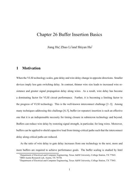
Chapter 26 <strong>Buffer</strong> <strong>Insertion</strong> <strong>Basics</strong><br />
Jiang Hu ∗ , Zhuo Li † and Shiyan Hu ‡<br />
1 Motivation<br />
When the VLSI technology scales, gate delay and wire delay change in opposite directions. Smaller<br />
devices imply less gate switching delay. In contrast, thinner wire size leads to increased wire resistance<br />
and greater signal propagation delay along wires. As a result, wire delay has become<br />
a dominating factor for VLSI circuit performance. Further, it is becoming a limiting factor to<br />
the progress of VLSI technology. This is the well-known interconnect challenge [1–3]. Among<br />
many techniques addressing this challenge [4, 5], buffer (or repeater) insertion is such an effective<br />
one that it is an indispensable necessity for timing closure in submicron technology and beyond.<br />
<strong>Buffer</strong>s can reduce wire delay by restoring signal strength, in particular, for long wires. Moreover,<br />
buffers can be applied to shield capacitive load from timing-critical paths such that the interconnect<br />
delay along critical paths are reduced.<br />
As the ratio of wire delay to gate delay increases from one technology to the next, more and<br />
more buffers are required to achieve performance goals. The buffer scaling is studied by Intel<br />
∗ Department of Electrical and <strong>Computer</strong> <strong>Engineering</strong>, Texas A&M University, College Station, TX 77843.<br />
† IBM Austin Research Lab, Austin, TX 78758.<br />
‡ Department of Electrical and <strong>Computer</strong> <strong>Engineering</strong>, Texas A&M University, College Station, TX 77843.<br />
1
and the results are reported in [6]. One metric that reveals the scaling is critical buffer length<br />
- the minimum distance beyond which inserting an optimally placed and sized buffer makes the<br />
interconnect delay less than that of the corresponding unbuffered wire. When wire delay increases<br />
due to the technology scaling, the critical buffer length becomes shorter, i.e., the distance that a<br />
buffer can comfortably drive shrinks. According to [6], the buffer critical length decreases by<br />
68% when the VLSI technology migrates from 90nm to 45nm (for two generations). Please note<br />
that the critical buffer length scaling significantly outpaces the VLSI technology scaling which is<br />
roughly 0.5× for every two generations. If we look at the percentage of block level nets requiring<br />
buffers, it grows from 5.8% in 90nm technology to 19.6% in 45nm technology [6]. Perhaps the<br />
most alarming result is the scaling of buffer count [6] which predicts that 35% of cells will be<br />
buffers in 45nm technology as opposed to only 6% in 90nm technology.<br />
The dramatic buffer scaling undoubtedly generates large and profound impact to VLSI circuit<br />
design. With millions of buffers required per chip, almost nobody can afford to neglect the importance<br />
of buffer insertion as compared to a decade ago when only a few thousands of buffers<br />
are needed for a chip [7]. Due to this importance, buffer insertion algorithms and methodologies<br />
need to be deeply studied on various aspects. First, a buffer insertion algorithm should deliver<br />
solutions of high quality since interconnect and circuit performance largely depend on the way<br />
that buffers are placed. Second, a buffer insertion algorithm needs to be sufficiently fast so that<br />
millions of nets can be optimized in reasonable time. Third, accurate delay models are necessary to<br />
ensure that buffer insertion solutions are reliable. Fourth, buffer insertion techniques are expected<br />
to simultaneously handle multiple objectives, such as timing, power and signal integrity, and their<br />
tradeoffs. Last but not the least, buffer insertion should interact with other layout steps, such as<br />
placement and routing, as the sheer number of buffers has already altered the landscape of circuit<br />
2
layout design. Many of these issues will be discussed in subsequent sections and other chapters.<br />
2 Optimization of Two-Pin Nets<br />
For buffer insertion, perhaps the most simple case is a two-pin net, which is a wire segment with a<br />
driver (source) at one end and a sink at the other end. The simplicity allows closed form solutions<br />
to buffer insertion in two-pin nets.<br />
If the delay of a two-pin net is to be minimized by using a single buffer type b, one needs to<br />
decide the number of buffers k and the spacing between the buffers, the source and the sink. First,<br />
let us look at a very simple case in order to attain an intuitive understanding of the problem. In this<br />
case, the length of the two-pin net is l and the wire resistance and capacitance per unit length are r<br />
and c, respectively. The number of buffers k has been given and is fixed. The driver resistance is<br />
the same as the buffer output resistance R b . The load capacitance of the sink is identical to buffer<br />
input capacitance C b . The buffer has an intrinsic delay of t b . The k buffers separates the net into<br />
k + 1 segments, with length of ⃗ l = (l 0 ,l 1 ,...,l k ) T (see Figure 1). Then, the Elmore delay of this<br />
net can be expressed as:<br />
t( ⃗ l) =<br />
k∑<br />
(αli 2 + βl i + γ) (1)<br />
i=0<br />
where α = 1 2 rc, β = R bc + rC b and γ = R b C b + t b . A formal problem formulation is<br />
Minimize t( ⃗ l) (2)<br />
Subject to<br />
g( ⃗ l) = l − ∑ k<br />
i=0 l i = 0 (3)<br />
According to the Kuhn-Tucker condition [8], the following equation is the necessary condition for<br />
3
the optimal solution.<br />
⃗∇t( ⃗ l) + λ ⃗ ∇g( ⃗ l) = 0 (4)<br />
where λ is the Lagrangian multiplier. According to the above condition, it can be easily derived<br />
that<br />
l i =<br />
β<br />
, i = 0, 1,...,k (5)<br />
λ − 2α<br />
Since α, β and λ are all constants, it can be seen that the buffers need to be equally spaced in order<br />
to minimize the delay. This is an important conclusion that can be treated as a rule of thumb. The<br />
value of the Lagrangian multiplier λ can be found by plugging (5) into (3).<br />
Driver<br />
l<br />
l l l<br />
2 3 k<br />
0 1 2 k<br />
1<br />
Sink<br />
Figure 1: <strong>Buffer</strong> insertion in a two-pin net.<br />
In more general cases, the driver resistance R d may be different from that of buffer output<br />
resistance and so is the sink capacitance C L . For such cases, the optimum number of buffers<br />
minimizing the delay is given by [9]:<br />
k =<br />
⌊− 1 2 + √<br />
1 + 2(rcl + r(C b − C L ) − c(R b − R d )) 2<br />
rc(R b C b + t b )<br />
⌋<br />
(6)<br />
4
The length of each segment can be obtained through [9]:<br />
(<br />
1<br />
k + 1<br />
l 0 = l + k(R b − R d )<br />
r<br />
l 1 = ... = l k−1 = 1<br />
k + 1<br />
l k =<br />
+ C )<br />
L − C b<br />
c<br />
(<br />
l − R b − R d<br />
r<br />
(<br />
1<br />
l − R b − R d<br />
− k(C L − C b )<br />
k + 1 r c<br />
+ C )<br />
L − C b<br />
c<br />
)<br />
(7)<br />
A closed form solution to simultaneous buffer insertion/sizing and wire sizing is reported in<br />
[10]. Figure 2 shows an example of this simultaneous optimization. The wire is segmented into<br />
m pieces. The length l i and width h i of each wire piece i are the variables to be optimized.<br />
There are k buffers inserted between these pieces. The size b i of each buffer i is also a decision<br />
variable. A buffer location is indicated by its surrounding wire pieces. For example, if the set<br />
of wire pieces between buffer i − 1 and i is P i−1 , the distance between the two buffers is equal<br />
to ∑ j∈P i−1<br />
l j . There are two important conclusions [10] for the optimal solution that minimizes<br />
the delay. First, all wire pieces have the same length, i.e., l i = l ,i = 1, 2,...,m. Second, for<br />
m<br />
wire pieces P i−1 = {p i−1,1 ,p i−1,2 ,...,p i−1,mi−1 } between buffer i − 1 and i, their widths satisfy<br />
h i−1,1 > h i−1,2 > ... > h i−1,mi−1 and form a geometric progression.<br />
m0 segments<br />
m k segments<br />
h 1 h 2 h m<br />
b 1 bk<br />
l 1 l 2<br />
l m<br />
Figure 2: An example of simultaneous buffer insertion/sizing and wire sizing.<br />
5
3 Van Ginneken’s algorithm<br />
For a general case of signal nets, which may have multiple sinks, van Ginneken’s algorithm [11]<br />
is perhaps the first systematic approach on buffer insertion. For a fixed signal routing tree and<br />
given candidate buffer locations, van Ginneken’s algorithm can find the optimal buffering solution<br />
that maximizes timing slack according to the Elmore delay model. If there are n candidate buffer<br />
locations, its computation complexity is O(n 2 ). Based on van Ginneken’s algorithm, numerous<br />
extensions have been made, such as handling of multiple buffer types, tradeoff with power and<br />
cost, addressing slew rate and crosstalk noise, using accurate delay models and speedup techniques.<br />
These extensions will be covered in subsequent sections.<br />
At a high level, van Ginneken’s algorithm [11] proceeds bottom-up from the leaf nodes toward<br />
the driver along a given routing tree. A set of candidate solutions keep updated during the process,<br />
where three operations adding wire, inserting buffers and branch merging may be performed.<br />
Meanwhile, the inferior solutions are pruned to accelerate the algorithm. After a set of candidate<br />
solutions are propagated to the source, the solution with the maximum required arrival time is<br />
selected as the final solution. For a routing tree with n buffer positions, the algorithm computes<br />
the optimal buffering solution in O(n 2 ) time.<br />
A net is given as a binary routing tree T = (V,E), where V = {s 0 }∪V s ∪V n , and E ⊆ V ×V .<br />
Vertex s 0 is the source vertex and also the root of T , V s is the set of sink vertices, and V n is the<br />
set of internal vertices. In the existing literatures, s 0 is also referred as driver. Denote by T(v)<br />
the subtree of T rooted at v. Each sink vertex s ∈ V s is associated with a sink capacitance C(s)<br />
and a required arrival time (RAT). Each edge e ∈ E is associated with lumped resistance R(e)<br />
and capacitance C(e). A buffer library B containing all the possible buffer types which can be<br />
6
assigned to a buffer position is also given. In this section, B contains only one buffer type. Delay<br />
estimation is obtained using the Elmore delay model, which is described in Chapter 3. A buffer<br />
assignment γ is a mapping γ : V n → B ∪{b} where b denotes that no buffer is inserted. The timing<br />
buffering problem is defined as follows.<br />
Timing Driven <strong>Buffer</strong> <strong>Insertion</strong> Problem: Given a binary routing tree T = (V,E), possible buffer<br />
positions, and a buffer library B, compute a buffer assignment γ such that the RAT at driver is<br />
maximized.<br />
3.1 Concept of Candidate Solution<br />
A buffer assignment γ is also called a candidate solution for the timing buffering problem. A<br />
partial solution, denoted by γ v , refers to an incomplete solution where the buffer assignment in<br />
T(v) has been determined.<br />
The Elmore delay from v to any sink s in T(v) under γ v is computed by<br />
D(s,γ v ) =<br />
∑<br />
(D(v i ) + D(e)),<br />
e=(v i ,v j )<br />
where the sum is taken over all edges along the path from v to s. The slack of vertex v under γ v is<br />
defined as<br />
Q(γ v ) = min {RAT(s) − D(s,γ v )}.<br />
s∈T(v)<br />
At any vertex v, the effect of a partial solution γ v to its upstream part is characterized by a<br />
(Q(γ v ),C(γ v )) pair, where Q is the slack at v under γ v and C is the downstream capacitance<br />
viewing at v under γ v .<br />
7
(a) Wire insertion.<br />
¤ ¢£ ¡<br />
(b) <strong>Buffer</strong> insertion.<br />
¦§¥¨ ¥<br />
<br />
(c) Branch merging.<br />
©<br />
Figure 3: Operations in van Ginneken’s algorithm.<br />
©<br />
3.2 Generating Candidate Solutions<br />
Van Ginneken’s algorithm proceeds bottom-up from the leaf nodes toward the driver along T . A set<br />
of candidate solutions, denoted by Γ, keep updated during this process. There are three operations<br />
through solution propagation, namely, wire insertion, buffer insertion and branch merging (see<br />
Figure 3). We are to describe them in turn.<br />
3.2.1 Wire insertion<br />
Suppose that a partial solution γ v at position v propagates to an upstream position u and there is no<br />
branching point in between. If no buffer is placed at u, then only wire delay needs to be considered.<br />
Therefore, the new solution γ u can be computed as<br />
Q(γ u ) = Q(γ v ) − D(e),<br />
C(γ u ) = C(γ v ) + C(e),<br />
(8)<br />
where e = (u,v) and D(e) = R(e)( C(e)<br />
2<br />
+ C(γ v )).<br />
8
3.2.2 <strong>Buffer</strong> insertion<br />
Suppose that we add a buffer b at u. γ u is then updated to γ ′ u where<br />
Q(γ ′ u) = Q(γ u ) − (R(b) · C(γ u ) + K(b)),<br />
C(γ ′ u) = C(b).<br />
(9)<br />
3.2.3 Branch merging<br />
When two branches T l and T r meet at a branching point v, Γ l and Γ r , which correspond to T l and<br />
T r , respectively, are to be merged. The merging process is performed as follows. For each solution<br />
γ l ∈ Γ l and each solution γ r ∈ Γ r , generate a new solution γ ′ according to:<br />
C(γ ′ ) = C(γ l ) + C(γ r ),<br />
Q(γ ′ ) = min{Q(γ l ),Q(γ r )}.<br />
(10)<br />
The smaller Q is picked since the worst-case circuit performance needs to be considered.<br />
3.3 Inferiority and Pruning Identification<br />
Simply propagating all solutions by the above three operations makes the solution set grow exponentially<br />
in the number of buffer positions processed. An effective and efficient pruning technique<br />
is necessary to reduce the size of the solution set. This motivates an important concept - inferior<br />
solution - in van Ginneken’s algorithm. For any two partial solutions γ 1 ,γ 2 at the same vertex v, γ 2<br />
is inferior to γ 1 if C(γ 1 ) ≤ C(γ 2 ) and Q(γ 1 ) ≥ Q(γ 2 ). Whenever a solution becomes inferior, it is<br />
pruned from the solution set. Therefore, only solutions excel in at least one aspect of downstream<br />
capacitance and slack can survive.<br />
9
For an efficient pruning implementation and thus an efficient buffering algorithm, a sorted list<br />
is used to maintain the solution set. The solution set Γ is increasingly sorted according to C, and<br />
thus Q is also increasingly sorted if Γ does not contain any inferior solutions.<br />
By a straightforward implementation, when adding a wire, the number of candidate solutions<br />
will not change; when inserting a buffer, only one new candidate solution will be introduced. More<br />
efforts are needed to merge two branches T l and T r at v. For each partial solution in Γ l , find the<br />
first solution with larger Q value in Γ r . If such a solution does not exist, the last solution in Γ r will<br />
be taken. Since Γ l and Γ r are sorted, we only need to traverse them once. Partial solutions in Γ r are<br />
similarly treated. It is easy to see that after merging, the number of solutions is at most |Γ l | + |Γ r |.<br />
As such, given n buffer positions, at most n solutions can be generated at any time. Consequently,<br />
the pruning procedure at any vertex in T runs in O(n) time.<br />
3.4 Pseudo-code<br />
In van Ginneken’s algorithm, a set of candidate solutions are propagated from sinks to driver.<br />
Along a branch, after a candidate buffer location v is processed, all solutions are propagated to<br />
its upstream buffer location u through wire insertion. A buffer is then inserted to each solution to<br />
obtain a new solution. Meanwhile, inferior solutions are pruned. At a branching point, solution<br />
sets from all branches are merged by merging process. In this way, the algorithm proceeds in<br />
the bottom-up fashion and the solution with maximum required arrival time at driver is returned.<br />
Given n buffer positions in T , van Ginneken’s algorithm can compute a buffer assignment with<br />
maximum slack at driver in O(n 2 ) time since any operation at any node can be performed in O(n)<br />
time. Refer to Figure 4 for the pseudo-code of van Ginneken’s algorithm.<br />
10
3.5 Example<br />
Algorithm: van Ginneken’s algorithm.<br />
Input: T : routing tree, B: buffer library<br />
Output: γ which maximizes slack at driver<br />
1. for each sink s, build a solution set {γ s }, where<br />
Q(γ s ) = RAT(s) and C(γ s ) = C(s)<br />
2. for each branching point/driver v t in the order given by<br />
a postorder traversal of T , let T ′ be each of the branches T 1 ,<br />
T 2 of v t and Γ ′ be the solution set corresponding to T ′ , do<br />
3. for each wire e in T ′ , in a bottom-up order, do<br />
4. for each γ ∈ Γ ′ , do<br />
5. C(γ) = C(γ) + C(e)<br />
6. Q(γ) = Q(γ) − D(e)<br />
7. prune inferior solutions in Γ ′<br />
8. if the current position allows buffer insertion, then<br />
9. for each γ ∈ Γ ′ , generate a new solution γ ′<br />
10. set C(γ ′ ) = C(b)<br />
11. set Q(γ ′ ) = Q(γ) − R(b) · C(γ) − K(b)<br />
12. Γ ′ = Γ ′ ⋃ {γ ′ } and prune inferior solutions<br />
13. // merge Γ 1 and Γ 2 to Γ vt<br />
14. set Γ vt = ∅<br />
15. for each γ 1 ∈ Γ 1 and γ 2 ∈ Γ 2 , generate a new solution γ ′<br />
16. set C(γ ′ ) = C(γ 1 ) + C(γ 2 )<br />
17. set Q(γ ′ ) = min{Q(γ 1 ),Q(γ 2 )}<br />
18. Γ vt = Γ vt<br />
⋃ {γ ′ } and prune inferior solutions<br />
19. return γ with the largest slack<br />
Figure 4: Van Ginneken’s algorithm.<br />
Let us look at a simple example to illustrate the work flow of van Ginneken’s algorithm. Refer to<br />
Figure 5. Assume that there are three non-dominated solutions at v 3 whose (Q,C) pairs are<br />
(200, 10), (300, 30), (500, 50),<br />
and there are two non-dominated solutions at v 2 whose (Q,C) pairs are<br />
(290, 5), (350, 20).<br />
11
Figure 5: An example for performing van Ginneken’s algorithm.<br />
<br />
We first propagate them to v 1 through wire insertion. Assume that R(v 1 ,v 3 ) = 3 and C(v 1 ,v 3 ) =<br />
<br />
2. Solution (200,10) at v 3 becomes (200 − 3 · (2/2 + 10), 10 + 2) = (167, 12) at v 1 . Similarly, the<br />
other two solutions become (207, 32), (347, 52). Assume that R(v 2 ,v 3 ) = 2 and C(v 2 ,v 3 ) = 2,<br />
solutions at v 2 become (278, 7), (308, 22) at v 1 .<br />
We are now to merge these solutions at v 1 . Denote by Γ l the solutions propagated from v 3 and<br />
by Γ r the solutions propagated from v 2 . Before merging, partial solutions in Γ l are<br />
(167, 12), (207, 32), (347, 52),<br />
and partial solutions in Γ r are<br />
(278, 7), (308, 22).<br />
After branch merging, the new candidate partial solutions whose Q are dictated by solutions in Γ l<br />
are<br />
(167, 19), (207, 39), (308, 74),<br />
12
and those dictated by solutions in Γ r are<br />
(278, 59), (308, 74).<br />
After pruning inferior solutions, the solution set at v 1 is<br />
{(167, 19), (207, 39), (278, 59), (308, 74)}.<br />
4 Van Ginneken Extensions<br />
4.1 Handling Library with Multiple <strong>Buffer</strong>s<br />
We extend the standard van Ginneken’s algorithm to handle multiple buffers and buffer cost [12].<br />
The buffer library B now contains various types of buffers. Each buffer b in the buffer library has<br />
a cost W(b), which can be measured by area or any other metric, depending on the optimization<br />
objective. A function f : V n → 2 B specifies the types of buffers allowed at each internal vertex in<br />
T . The cost of a solution γ, denoted by W(γ), is defined as W(γ) = ∑ b∈γ W b. With the above<br />
notations, our new problem can be formulated as follows.<br />
Minimum Cost Timing Constrained <strong>Buffer</strong> <strong>Insertion</strong> Problem: Given a binary routing tree T =<br />
(V,E), possible buffer positions defined using f, and a buffer library B, to compute a minimalcost<br />
buffer assignment γ such that the RAT at driver is smaller than a timing constraint α.<br />
In contrast to the single buffer type case, W is introduced into the (Q,C) pair to handle buffer<br />
cost, i.e., each solution is now associated with a (Q,C,W)-triple. As such, during the process of<br />
bottom-up computation, additional efforts need to be made in updating W : if γ ′ is generated by<br />
13
inserting a wire into γ, then W(γ ′ ) = W(γ); if γ ′ is generated by inserting a buffer b into γ, then<br />
W(γ ′ ) = W(γ) + W(b); if γ ′ is generated by merging γ l with γ r , then W(γ ′ ) = W(γ l ) + W(γ r ).<br />
The definition of inferior solutions needs to be revised as well. For any two solutions γ 1 ,γ 2 at<br />
the same node, γ 1 dominates γ 2 if C(γ 1 ) ≤ C(γ 2 ), W(γ 1 ) ≤ W(γ 2 ) and Q(γ 1 ) ≥ Q(γ 2 ). Whenever<br />
a solution becomes dominated, it is pruned from the solution set. Therefore, only solutions<br />
excel in at least one aspect of downstream capacitance, buffer cost and RAT can survive.<br />
With the above modification, van Ginneken’s algorithm can easily adapt to the new problem<br />
setup. However, since the domination is defined on a (Q,C,W) triple rather than a (Q,C) pair,<br />
more efficient pruning technique is necessary to maintain the efficiency of the algorithm. As such,<br />
range search tree technique is incorporated [12]. This technique will be described in details in<br />
Section 5.2.<br />
4.2 Library with Inverters<br />
So far, all buffers in the buffer library are non-inverting buffers. There can also have inverting<br />
buffers, or simply inverters. In terms of buffer cost and delay, inverter would provide cheaper<br />
buffer assignment and better delay over non-inverting buffers. As regard to algorithmic design,<br />
it is worth noting that introducing inverters into the buffer library brings the polarity issue to the<br />
problem, as the output polarity of a buffer will be negated after inserting an inverter.<br />
4.3 Polarity Constraints<br />
When output polarity for driver is required to be positive or negative, we impose a polarity constraint<br />
to the buffering problem. To handle polarity constraints, during the bottom-up computation,<br />
14
the algorithm maintains two solution sets, one for positive and one for negative buffer input polarity.<br />
After choosing the best solution at driver, the buffer assignment can be then determined by a<br />
top-down traversal. The details of the new algorithm are elaborated as follows.<br />
Denote the two solution sets at vertex v by Γ + v and Γ − v corresponding to positive polarity and<br />
negative polarity, respectively. Supposed that an inverter b − is inserted to a solution γ v + ∈ Γ + v ,<br />
a new solution γ v ′ is generated in the same way as before except that it will be placed into Γ − v .<br />
Similarly, the new solution generated by inserting b − to a solution γv − ∈ Γ − v will be placed into Γ + v .<br />
For inserting a non-inverting buffer, the new solution is placed in the same set as its origin.<br />
The other operations are easier to handle. The wire insertion goes the same as before and two<br />
solution sets are handled separately. Merging is carried out only among the solutions with the same<br />
polarity, e.g., the positive-polarity solution set of left branch is merged with that of the right branch.<br />
For inferiority check and solution pruning, only the solutions in the same set can be compared.<br />
4.4 Slew and Capacitance Constraints<br />
The slew rate of a signal refers to the rising or falling time of a signal switching. Sometimes<br />
the slew rate is referred as signal transition time. The slew rate of almost every signal has to be<br />
sufficiently small since a large slew rate implies large delay, large short circuit power dissipation<br />
and large vunlerability to crosstalk noise. In practice, a maximal slew rate constraint is required<br />
at the input of each gate/buffer. Therefore, this constraint needs to be obeyed in a buffering algorithm<br />
[12–15].<br />
A simple slew model is essentially equivalent to the Elmore model for delay. It can be explained<br />
using a generic example which is a path p from node v i (upstream) to v j (downstream) in a buffered<br />
15
tree. There is a buffer (or the driver) b u at v i , and there is no buffer between v i and v j . The slew<br />
rate S(v j ) at v j depends on both the output slew S bu,out(v i ) at buffer b u and the slew degradation<br />
S w (p) along path p (or wire slew), and is given by [16]:<br />
S(v j ) =<br />
√<br />
S bu,out(v i ) 2 + S w (p) 2 . (11)<br />
The slew degradation S w (p) can be computed with Bakoglu’s metric [17] as<br />
S w (p) = ln 9 · D(p), (12)<br />
where D(p) is the Elmore delay from v i to v j .<br />
The output slew of a buffer, such as b u at v i , depends on the input slew at this buffer and the<br />
load capacitance seen from the output of the buffer. Usually, the dependence is described as a 2-D<br />
lookup table. As a simplified alternative, one can assume a fixed input slew at each gate/buffer.<br />
This fixed slew is equal to the maximum slew constraint and therefore is always satisfied but is a<br />
conservative estimation. For fixed input slew, the output slew of buffer b at vertex v is then given<br />
by<br />
S b,out (v) = R b · C(v) + K b , (13)<br />
where C(v) is the downstream capacitance at v, R b and K b are empirical fitting parameters. This<br />
is similar to empirically derived K-factor equations [18]. We call R b the slew resistance and K b<br />
the intrinsic slew of buffer b.<br />
In a van Ginneken style buffering algorithm, if a candidate solution has a slew rate greater than<br />
16
given slew constraint, it is pruned out and will not be propagated any more. Similar as the slew<br />
constraint, circuit designs also limit the maximum capacitive load a gate/buffer can drive [15]. For<br />
timing non-critical nets, buffer insertion is still necessary for the sake of satisfying the slew and<br />
capacitance constraints. For this case, fast slew buffering techniques are introduced in [19].<br />
4.5 Integration with Wire Sizing<br />
In addition to buffer insertion, wire sizing is an effective technique for improving interconnect<br />
performance [20–24]. If wire size can take only discrete options, which is often the case in practice,<br />
wire sizing can be directly integrated with van Ginneken style buffer insertion algorithm [12]. In<br />
the bottom-up dynamic programming procedure, multiple wire width options need to be considered<br />
when a wire is added (see Section 3.2.1). If there are k options of wire size, then k new candidate<br />
solutions are generated, one corresponding each wire size. However, including the wire sizing in<br />
van Ginneken’s algorithm makes the complexity pseudo-polynomial [12].<br />
In [25], layer assignment and wire spacing are considered in conjunction with wire sizing. A<br />
combination of layer, width and spacing is called a wire code. All wires in a net have to use an<br />
identical wire code. If each wire code is treated as a polarity, the wire code assignment can be<br />
integrated with buffer insertion in the same way as handling polarity constraint (see Section 4.3).<br />
In contrast to simultaneous wire sizing and buffer insertion [12], the algorithm complexity stays<br />
polynomial after integrating wire code assignment [25] with van Ginneken’s algorithm.<br />
Another important conclusion in [25] is about wire tapering. Wire tapering means that a wire<br />
segment is divided into multiple pieces and each piece can be sized individually. In contrast,<br />
uniform wire sizing does not make such division and maintain the same wire width for the entire<br />
17
Tapered Wire Sizing<br />
Uniform Wire Sizing<br />
Figure 6: Wire sizing with tapering and uniform wire sizing.<br />
segment. These two cases are illustrated in Figure 6. It is shown in [25] that the benefit of wire<br />
tapering versus uniform wire sizing is very limited when combined with buffer insertion. It is<br />
theoretically proved [25] that the signal velocity from simultaneous buffering with wire tapering<br />
is at most 1.0354 times of that from buffering and uniform wire sizing. In short, wire tapering<br />
improves signal speed by at most 3.54% over uniform wire sizing.<br />
4.6 Noise Constraints with Devgan Metric<br />
The shrinking of minimum distance between adjacent wires has caused an increase in the coupling<br />
capacitance of a net to its neighbors. A large coupling capacitance can cause a switching net<br />
to induce significant noise onto a neighboring net, resulting in an incorrect functional response.<br />
Therefore, noise avoidance techniques must become an integral part of the performance optimization<br />
environment.<br />
The amount of coupling capacitance from one net to another is proportional to the distance that<br />
the two nets run parallel to each other. The coupling capacitance may cause an input signal on<br />
the aggressor net to induce a noise pulse on the victim net. If the resulting noise is greater than<br />
18
the tolerable noise margin (NM) of the sink, then an electrical fault results. Inserting buffers in<br />
the victim net can separate the capacitive coupling into several independent and smaller portions,<br />
resulting in smaller noise pulse on the sink and the input of the inserted buffers.<br />
Before describing the noise-aware buffering algorithms, we first introduce the coupling noise<br />
metric in Section 4.6.1.<br />
4.6.1 Devgan’s coupling noise metric<br />
Among many coupling noise models, Devgan’s metric [26] is particularly amenable for noise<br />
avoidance in buffer insertion, because its computational complexity, structure, and incremental<br />
nature is the same as the famous Elmore delay metric. Further, like the Elmore delay model, the<br />
noise metric is a provable upper bound on coupled noise. Other advantages of the noise metric<br />
include the ability to incorporate multiple aggressor nets and handle general victim and aggressor<br />
net topologies. A disadvantage of the Devgan metric is that it becomes more pessimistic as the ratio<br />
of the aggressor net’s transition time (at the output of the driver) to its delay decreases. However,<br />
cases in which this ratio becomes very small are rare since a long net delay generally corresponds<br />
to a large load on the driver, which in turn causes a slower transition time. The metric does not<br />
consider the duration of the noise pulse either. In general, the noise margin of a gate is dependent<br />
on both the peak noise amplitude and the noise pulse width. However, when considering failure at<br />
a gate, peak amplitude dominates pulse width.<br />
If a wire segment e in the victim net is adjacent with t aggressor nets, let λ 1 ,...,λ t be the ratios<br />
of coupling to wire capacitance from each aggressor net to e, and let µ 1 ,...,µ t be the slopes of the<br />
aggressor signals. The impact of a coupling from aggressor j can be treated as a current source<br />
I e,j = C e ·λ j ·µ j where C e is the wire capacitance of wire segment e. This is illustrated in Figure 7.<br />
19
(a)<br />
(b)<br />
Figure 7: Illustration of noise model.<br />
The total current induced by the aggressors on e is<br />
t∑<br />
I e = C e (λ j · µ j ) (14)<br />
j=1<br />
Often, information about neighboring aggressor nets is unavailable, especially if buffer insertion<br />
is performed before routing. In this case, a designer may wish to perform buffer insertion<br />
to improve performance while also avoiding future potential noise problems. When performing<br />
buffer insertion in estimation mode, one might assume that: (1) there is a single aggressor net<br />
which couples with each wire in the routing tree, (2) the slope of all aggressors is µ, and (3) some<br />
fixed ratio λ of the total capacitance of each wire is due to coupling capacitance.<br />
Let I T(v) be defined as the total downstream current see at node v, i.e.,<br />
I T(v) = ∑<br />
e∈E T(v)<br />
Ie,<br />
where E T(v) is the set of wire edges downstream of node v. Each wire adds to the noise induced<br />
on the victim net. The amount of additional noise induced from a wire e = (u,v) is given by<br />
Noise(e) = R e ( I e<br />
2 + I T(v)) (15)<br />
20
where R e is the wire resistance. The total noise seen at sink si starting at some upstream node v is<br />
∑<br />
Noise(v − si) = R v I T(v) + Noise(e) (16)<br />
e∈path(v−si)<br />
where R v = 0 if there is no gate at node v. The path from v to si has no intermediate buffers.<br />
Each node v has a predetermined noise margin NM(v). If the circuit is to have no electrical<br />
faults, the total noise propagated from each driver/buffer to each its sink si must be less than the<br />
noise margin for si. We define the noise slack for every node v as<br />
NS(v) =<br />
min NM(si) − Noise(v − si) (17)<br />
si∈SI T(v)<br />
where SI T(v) is the set of sink nodes for the subtree rooted at node v. Observe that NS(si) =<br />
NM(si) for each sink si.<br />
4.6.2 Algorithm of buffer insertion with noise avoidance<br />
We begin with the simplest case of a single wire with uniform width and neighboring coupling<br />
capacitance. Let us consider a wire e = (u,v). First, we need to ensure NS(v) ≥ R b I T(v) where<br />
R b is the buffer output resistance. If this condition is not satisfied, inserting a buffer even at node<br />
v cannot satisfy the constraint of noise margin, i.e., buffer insertion is needed within subtree T(v).<br />
If NS(v) ≥ R b I T(v) , we next search for the maximum wirelength l e,max of e such that inserting a<br />
buffer at u always satisfies noise constraints. The value of l e,max tells us the maximum unbuffered<br />
length or the minimum buffer usage for satisfying noise constraints. Let R = R e /l e be the wire<br />
resistance per unit length and I = I e /l e be the current per unit length. According to [27], this value<br />
21
can be determined by<br />
l e,max = − R b<br />
R − I T(v)<br />
+<br />
I<br />
√<br />
( R b<br />
R )2 + ( I T(v)<br />
)<br />
I<br />
2 + 2NS(v)<br />
I · R<br />
(18)<br />
Depending on the timing criticality of the net, the noise-aware buffer insertion problem can be<br />
formulated in two different ways: (A) minimize total buffer cost subject to noise constraints; (B)<br />
maximize timing slack subject to noise constraints.<br />
The algorithm for (A) is a bottom-up dynamic programming procedure which inserts buffers<br />
greedily as far apart as possible [27]. Each partial solution at node v is characterized by a 3-tuple<br />
of downstream noise current I T(v) , noise slack NS(v) and buffer assignment M. In the solution<br />
propagation, the noise current is accumulated in the same way as the downstream capacitance in<br />
van Ginneken’s algorithm. Likewise, noise slack is treated like the timing slack (or required arrival<br />
time). This algorithm can return an optimal solution for a multi-sink tree T = (V,E) in O(|V | 2 )<br />
time.<br />
The core algorithm of noise constrained timing slack maximization is similar as van Ginneken’s<br />
algorithm except that the noise constraint is considered. Each candidate solution at node v is<br />
represented by a 5-tuple of downstream capacitance C v , required arrival time q(v), downstream<br />
noise current I T(v) , noise slack NS(v) and buffer assignment M. In addition to pruning inferior<br />
solutions according to the (C,q) pair, the algorithm eliminates candidate solutions that violate the<br />
noise constraint. At the source, the buffering solution not only has optimized timing performance<br />
but also satisfies the noise constraint.<br />
22
4.7 Higher Order Delay Modeling<br />
Many buffer insertion methods [11, 12, 28] are based on the Elmore wire delay model [29] and<br />
a linear gate delay model for the sake of simplicity. However, the Elmore delay model often<br />
overestimates interconnect delay. It is observed in [30] that Elmore delay sometimes has over<br />
100% overestimation error when compared to SPICE. A critical reason of the overestimation is<br />
due to the neglection of the resistive shielding effect. In the example of Figure 8, the Elmore delay<br />
from node A to B is equal to R 1 (C 1 + C 2 ) assuming that R 1 can see the entire capacitance of C 2<br />
despite the fact that C 2 is somewhat shielded by R 2 . Consider an extreme scenario where R 2 = ∞<br />
or there is open circuit between node B and C. Obviously, the delay from A to B should be R 1 C 1<br />
instead of the Elmore delay R 1 (C 1 + C 2 ). The linear gate delay model is inaccurate due to its<br />
neglection of nonlinear behavior of gate delay in addition to resistive shielding effect. In other<br />
words, a gate delay is not a strictly linear function of load capacitance.<br />
A<br />
R 1 R 2<br />
C 2<br />
C 1<br />
B C<br />
Figure 8: Example of resistive shielding effect.<br />
The simple and relatively inaccurate delay models are suitable only for early design stages<br />
such as buffer planning. In post-placement stages, more accurate models are needed because (1)<br />
optimal buffering solutions based on simple models may be inferior since actual delay is not being<br />
optimized; (2) simplified delay modeling can cause a poor evaluation of the trade-off between total<br />
buffer cost and timing improvement. In more accurate delay models, the resistive shielding effect<br />
is considered by replacing lumped load capacitance with higher order load admittance estimation.<br />
23
The accuracy of wire delay can be improved by including higher order moments of transfer function.<br />
An accurate and popular gate delay model is usually a lookup table employed together with<br />
effective capacitance [31, 32] which is obtained based on the higher order load admittance. These<br />
techniques will be described in more details as follows.<br />
4.7.1 Higher order point admittance model<br />
For an RC tree, which is a typical circuit topology in buffer insertion, the frequency domain point<br />
admittance at a node v is denoted as Y v (s). It can be approximated by the third order Taylor<br />
expansion<br />
Y v (s) = y v,0 + y v,1 s + y v,2 s 2 + y v,3 s 3 + O(s 4 )<br />
where y v,0 , y v,1 , y v,2 and y v,3 are expansion coefficients. The third order approximation usually<br />
provides satisfactory accuracy in practice. Its computation is a bottom-up procedure starting from<br />
the leaf nodes of an RC tree, or the ground capacitors. For a capacitance C connected to ground,<br />
the admittance at its upstream end is simply Cs. Please note that the zeroth order coefficient is<br />
equal to 0 in an RC tree since there is no DC path connected to ground. Therefore, we only need<br />
to propagate y 1 , y 2 and y 3 in the bottom-up computation. There are two cases we need to consider:<br />
• Case 1: For a resistance R, given the admittance Y d (s) of its downstream node, compute the<br />
admittance Y u (s) of its upstream node (Figure 9(a)).<br />
y u,1 = y d,1 y u,2 = y d,2 − Ry 2 d,1 y u,3 = y d,3 − 2Ry d,1 y d,2 + R 2 y 3 d,1 (19)<br />
• Case 2: Given admittance Y d1 (s) and Y d2 (s) corresponding to two branches, compute the<br />
24
admittance Y u (s) after merging them (Figure 9(b)).<br />
y u,1 = y d1,1 + y d2,1 y u,2 = y d1,2 + y d2,2 y u,3 = y d1,3 + y d2,3 (20)<br />
Y (s) d1<br />
Y u(s)<br />
R<br />
Y (s) d<br />
Y (s) u<br />
Y (s) d2<br />
(a)<br />
(b)<br />
Figure 9: Two scenarios of admittance propagation.<br />
The third order approximation (y 1 ,y 2 ,y 3 ) of an admittance can be realized as an RC π−model<br />
(C u ,R π ,C d ) (Figure 10)where<br />
C u = y 1 − y2 2<br />
y 3<br />
R π = − y2 3<br />
y 3 2<br />
C d = y2 2<br />
y 3<br />
(21)<br />
Y(s)<br />
R π<br />
C<br />
u<br />
C d<br />
Figure 10: Illustration of π−model.<br />
4.7.2 Higher order wire delay model<br />
While the Elmore delay is equal to the first order moment of transfer function, the accuracy of<br />
delay estimation can be remarkably improved by including higher order moments. For example,<br />
25
the wire delay model [33] based on the first three moments and the closed-form model [34] using<br />
the first two moments.<br />
Since van Ginneken style buffering algorithms proceed in a bottom-up manner, bottom-up<br />
moment computations are required. Figure 11(a) shows a wire e connected to a subtree rooted at<br />
node B. Assume that the first k moments m (1)<br />
BC , m(2) BC<br />
, ..., m(k)<br />
BC<br />
have already been computed for<br />
the path from B to C. We wish to compute the moments m (1)<br />
AC , m(2) AC<br />
, ..., m(k)<br />
AC<br />
so that the A ❀ C<br />
delay can be derived.<br />
A<br />
wire e<br />
R e , Ce<br />
B<br />
C<br />
R e<br />
A<br />
Ce /2 C e /2<br />
B<br />
C j<br />
R π<br />
C f<br />
D<br />
A<br />
/2 C e<br />
R e<br />
B<br />
C n<br />
R π<br />
C f<br />
D<br />
(a)<br />
Figure 11: Illustration of bottom-up moment computation.<br />
(b)<br />
(c)<br />
The techniques in Section 4.7.1 are used to reduce the subtree at B to a π− model (C j ,R π ,C f )<br />
(Figure 11(b)). Node D just denotes the point on the far side of the resistor connected to B and<br />
is not an actual physical location. The RC tree can be further simplified to the network shown in<br />
Figure 11(c). The capacitance C j and C e /2 at B are merged to form a capacitor with value C n .<br />
The moments from A to B can be recursively computed by the equation<br />
m (i)<br />
AB = −R e(m (i−1)<br />
AB<br />
+ m(i−1) AD C f) (22)<br />
where the moments from A to D are given by<br />
m (i)<br />
AD = m(i) AB − m(i−1) AD R πC f (23)<br />
26
and m (0)<br />
AB = m(0) AD<br />
= 1. Now the moments from A to C can be computed via moment multiplication<br />
as follows.<br />
m (i)<br />
AC = i∑<br />
(m (j)<br />
AB · m(i−j)<br />
j=0<br />
BC ) (24)<br />
One property of Elmore delay that makes it attractive for timing optimization is that the delays<br />
are additive. This property does not hold for higher order delay models. Consequently, a<br />
non-critical sink in a subtree may become a critical sink depending the value of upstream resistance<br />
[35]. Therefore, one must store the moments for all the paths to downstream sinks during the<br />
bottom-up candidate solution propagation.<br />
4.7.3 Accurate gate delay<br />
A popular gate delay model with decent accuracy consists of the following three steps:<br />
1. Compute a π−model of the driving point admittance for the RC interconnect using the techniques<br />
introduced in Section 4.7.1.<br />
2. Given the π−model and the characteristics of the driver, compute an effective capacitance<br />
C eff [31, 32].<br />
3. Based on C eff , compute the gate delay using k−factor equations or lookup table [36].<br />
4.8 Flip-flop <strong>Insertion</strong><br />
The technology scaling leads to decreasing clock period, increasing wire delay and growing chip<br />
size. Consequently, it often takes multiple clock cycles for signals to reach their destinations along<br />
global wires. Traditional interconnect optimization techniques such as buffer insertion are inade-<br />
27
quate in handling this scenario and flip-flop/latch insertion (or interconnect pipelining) becomes a<br />
necessity.<br />
In pipelined interconnect design, flip-flops and buffers are inserted simultaneously in a given<br />
Steiner tree T = (V,E) [37,38]. The simultaneous insertion algorithm is similar to van Ginneken’s<br />
dynamic programming method except that a new criterion - latency, needs to be considered. The latency<br />
from the signal source to a sink is the number of flip-flops in-between. Therefore, a candidate<br />
solution at node v ∈ V is characterized by its latency λ v in addition to downstream capacitance<br />
C v , required arrival time (RAT) q v . Obviously, a small latency is preferred.<br />
The inclusion of flip-flop and latency also requests other changes in a van Ginneken style<br />
algorithm. When a flip-flop is inserted in the bottom-up candidate propagation, the RAT at the<br />
input of this flip-flop is reset to clock period time T φ . The latency of corresponding candidate<br />
solution is also increased by 1. For the ease of presentation, clock skew and setup/hold time are<br />
neglected without loss of generality. Then, the delay between two adjacent flip-flops cannot be<br />
greater than the clock period time T φ , i.e., the RAT cannot be negative. During the candidate<br />
solution propagation, if a candidate solution has negative RAT, it should be pruned without further<br />
propagation. When merge two candidate solutions from two child branches, the latency of the<br />
merged solution is the maximum of the two branch solutions.<br />
There are two formulations for the simultaneous flip-flop and buffer insertion problem. MiLa:<br />
find the minimum latency that can be obtained. GiLa: find a flip-flop/buffer insertion implementation<br />
that satisfies given latency constraint. MiLa can be used for the estimation of interconnect<br />
latency at the micro architectural level. After the micro-architecture design is completed, all interconnect<br />
must be designed so as to abide to given latency requirements by using GiLa.<br />
The algorithm of MiLa [38] and GiLa [38] are shown in Figure 12 and Figure 13, respectively.<br />
28
In GiLa, the λ u for a leaf node u is the latency constraint at that node. Usually, λ u at a leaf is<br />
a non-positive number. For example, λ u = −3 requires that the latency from the source to node<br />
u is 3. During the bottom-up solution propagation, λ is increased by 1 if a flip-flop is inserted.<br />
Therefore, λ = 0 at the source implies that the latency constraint is satisfied. If the latency at the<br />
source is greater than zero, then the corresponding solution is not feasible (line 2.6.1 of Figure 13).<br />
If the latency at the source is less than zero, the latency constraint can be satisfied by padding<br />
extra flip-flops in the corresponding solution (line 2.6.2.1 of Figure 13). The padding procedure<br />
is called ReFlop(T u ,k) which inserts k flip-flops in the root path of T u . The root path is from<br />
u to either a leaf node or a branch node v and there is no other branch node in-between. The<br />
flip-flops previously inserted on the root path and the newly inserted k flip-flops are redistributed<br />
evenly along the path. When merge solutions from two branches in GiLa, ReFlop is performed<br />
(line 3.3-3.4.1 of Figure 13) for the solutions with smaller latency to ensure that there is at least<br />
one merged solution matching the latency of both branches.<br />
5 Speedup Techniques<br />
Due to dramatically increasing number of buffers inserted in the circuits, algorithms that can efficiently<br />
insert buffers are essential for the design automation tools. In this chapter, several recent<br />
proposed speedup results are introduced and the key techniques are described.<br />
5.1 Recent Speedup Results<br />
This chapter studies buffer insertion in interconnect with a set of possible buffer positions and a<br />
discrete buffer library. In 1990, van Ginneken [11] proposed an O(n 2 ) time dynamic programming<br />
29
Algorithm: MiLa(T u )/MiLa(T u,v )<br />
Input: Subtree rooted at node u or edge (u, v)<br />
Output: A set of candidate solutions Γ u<br />
Global: Routing tree T and buffer library B<br />
1. if u is a leaf, Γ u = (C u , q u , 0, 0) // q is required arrival time<br />
2. else if u has one child node v or the input is T u,v<br />
2.1 Γ v = MiLa(v)<br />
2.2 Γ u = ∪ γ∈Γv (addWire((u, v), γ))<br />
2.3 Γ b = ∅<br />
2.4 for each b in B<br />
2.4.1 Γ = ∪ γ∈Γu (add<strong>Buffer</strong>(γ, b))<br />
2.4.2 prune Γ<br />
2.4.3 Γ b = Γ b ∪ Γ<br />
2.5 Γ u = Γ u ∪ Γ b<br />
3. else if u has two child edges (u, v) and (u, z)<br />
3.1 Γ u,v = MiLa(T u,v ), Γ u,z = MiLa(T u,z )<br />
3.2 Γ u = Γ u ∪ merge(Γ u,v , Γ u,z )<br />
4. prune Γ u<br />
5. return Γ u<br />
Figure 12: The MiLa algorithm.<br />
algorithm for buffer insertion with one buffer type, where n is the number of possible buffer positions.<br />
His algorithm finds a buffer insertion solution that maximizes the slack at the source. In<br />
1996, Lillis, Cheng and Lin [12] extended van Ginneken’s algorithm to allow b buffer types in time<br />
O(b 2 n 2 ).<br />
Recently, many efforts are taken to speedup the van Ginneken’s algorithm and its extension.<br />
Shi and Li [39] improved the time complexity of van Ginneken’s algorithm to O(b 2 n log n) for<br />
2-pin nets, and O(b 2 n log 2 n) for multi-pin nets. The speedup is achieved by four novel techniques:<br />
predictive pruning, candidate tree, fast redundancy check, and fast merging. To reduce the<br />
quadratic effect of b, Li and Shi [40] proposed an algorithm with time complexity O(bn 2 ). The<br />
speedup is achieved by the observation that the best candidate to be associated with any buffer<br />
must lie on the convex hull of the (Q,C) plane and convex pruning. To utilize the fact that in real<br />
applications most nets have small numbers of pins and large number of buffer positions, Li and<br />
30
Algorithm: GiLa(T u )/GiLa(T u,v )<br />
Input: Subtree T u rooted at node u or edge (u, v)<br />
Output: A set of candidate solutions Γ u<br />
Global: Routing tree T and buffer library B<br />
1. if u is a leaf, Γ u = (C u , q u , λ u , 0)<br />
2. else if node u has one child node v or the input is T u,v<br />
2.1 Γ v = GiLa(T v )<br />
2.2 Γ u = ∪ γ∈Γv (addWire((u, v), γ))<br />
2.3 Γ b = ∅<br />
2.4 for each b in B<br />
2.4.1 Γ = ∪ γ∈Γu (add<strong>Buffer</strong>(γ, b))<br />
2.4.2 prune Γ<br />
2.4.3 Γ b = Γ b ∪ Γ<br />
2.5 Γ u = Γ u ∪ Γ b<br />
// Γ u ≡ {Γ x , ...,Γ y }, x, y indicate latency<br />
2.6 if u is source<br />
2.6.1 if x > 0, exit: the net is not feasible<br />
2.6.2 if y < 0, // insert −y more flops in Γ u<br />
2.6.2.1 Γ u = ReFlop(T u , −y)<br />
3. else if u has two child edges (u, v) and (u, z)<br />
3.1 Γ u,v = GiLa(T u,v ), Γ u,z = GiLa(T u,z )<br />
3.2 //Γ u,v ≡ {Γ x , ...,Γ y }, Γ u,z ≡ {Γ m , ...,Γ n }<br />
3.3 if y < m // insert m − y more flops in Γ u,v<br />
3.3.1 Γ u,v = ReFlop(T u,v , m − y)<br />
3.4 if n < x // insert x − n more flops in Γ u,z<br />
3.4.1 Γ u,z = ReFlop(T u,z , x − n)<br />
3.5 Γ u = Γ u ∪ merge(Γ u,v , Γ u,z )<br />
4. prune Γ u<br />
5. return Γ u<br />
Figure 13: The GiLa algorithm.<br />
Shi [41] proposed a simple O(mn) algorithms for m-pin nets. The speedup is achieved by the<br />
property explored in [40], convex pruning, a clever bookkeeping method and an innovative linked<br />
list that allow O(1) time update for adding a wire or a candidate.<br />
In the following subsections, new pruning techniques, efficient way to find the best candidates<br />
when adding a buffer, and implicit data representations are presented. They are the basic component<br />
of many recent speedup algorithms.<br />
31
5.2 Predictive Pruning<br />
During the van Ginneken’s algorithm, a candidate is pruned out only if there is another candidate<br />
that is superior in terms of capacitance and slack. This pruning is based on the information at<br />
the current node being processed. However, all candidates at this node must be propagated further<br />
upstream toward the source. This means the load seen at this node must be driven by some minimal<br />
amount of upstream wire or gate resistance. By anticipating the upstream resistance ahead of time,<br />
one can prune out more potentially inferior candidates earlier rather than later, which reduces the<br />
total number of candidates generated. More specifically, assume that each candidate must be driven<br />
by an upstream resistance of at least R min . The pruning based on anticipated upstream resistance<br />
is called predictive pruning.<br />
Definition 1 (Predictive pruning) Let α 1 and α 2 be two nonredundant candidates of T(v) such<br />
that C(α 1 ) < C(α 2 ) and Q(α 1 ) < Q(α 2 ). If Q(α 2 ) − R min · C(α 2 ) ≤ Q(α 1 ) − R min · C(α 1 ),<br />
then α 2 is pruned.<br />
Predictive pruning preserves optimality. The general situation is shown in Fig. 14. Let α 1 and<br />
α 2 be candidates of T(v 1 ) that satisfy the condition in Definition 1. Using α 1 instead of α 2 will<br />
not increase delay from v to sinks in v 2 ,...,v k . It is easy to see C(v,α 1 ) < C(v,α 2 ). If Q at v is<br />
determined by T(v 1 ), we have<br />
Q(v,α 1 ) − Q(v,α 2 ) = Q(v 1 ,α 1 ) − Q(v 1 ,α 2 ) − R min · (C(v 1 ,α 1 ) − C(v 1 ,α 2 ))<br />
≥ 0<br />
Therefore, α 2 is redundant.<br />
32
v<br />
R min<br />
v 2<br />
v 3 ... v k<br />
v 1<br />
T(v 1<br />
)<br />
Figure 14: If α 1 and α 2 satisfy the condition in Definition 1 at v 1 , α 2 is redundant.<br />
Predictive pruning technique prunes more redundant solutions while guarantees optimality. It<br />
is one of four key techniques of fast algorithms proposed in [39]. In [42], significant speedup is<br />
achieved by simply extending predictive pruning technique to buffer cost. Aggressive predictive<br />
pruning technique, which uses a resistance larger than R min to prune candidates, is proposed in [43]<br />
to achieve further speedup with a little degradation of solution quality.<br />
5.3 Convex Pruning<br />
The basic data structure of van Ginneken’s algorithms is a sorted list of non-dominated candidates.<br />
Both the pruning in van Ginneken’s algorithm and the predictive pruning are performed by comparing<br />
two neighboring candidates a time. However, more potentially inferior candidates can be<br />
pruned out by comparing three neighboring candidate solutions simultaneously. For three solutions<br />
in the sorted list, the middle one may be pruned according to convex pruning.<br />
Definition 2 (Convex pruning) Let α 1 ,α 2 and α 3 be three nonredundant candidates of T(v) such<br />
that C(α 1 ) < C(α 2 ) < C(α 3 ) and Q(α 1 ) < Q(α 2 ) < Q(α 3 ). If<br />
Q(α 2 ) − Q(α 1 )<br />
C(α 2 ) − C(α 1 ) < Q(α 3) − Q(α 2 )<br />
C(α 3 ) − C(α 2 ) , (25)<br />
then we call α 2 non-convex, and prune it.<br />
33
Convex pruning can be explained by Figure 15. Consider Q as the Y -axis and C as the X-axis.<br />
Then candidates are points in the two-dimensional plane. It is easy to see that the set of nonredundant<br />
candidates N(v) is a monotonically increasing sequence. Candidate α 2 = (Q 2 ,C 2 ) in the<br />
above definition is shown in Figure 15(a), and is pruned in Figure 15(b). The set of nonredundant<br />
candidates after convex pruning M(v) is a convex hull.<br />
q<br />
q<br />
q 4<br />
q 3<br />
Pruned<br />
q 4<br />
q 3<br />
q 2<br />
q 1<br />
c 1<br />
c 2<br />
c 3<br />
c 4<br />
c<br />
q 1<br />
c 1<br />
c 3<br />
c 4<br />
c<br />
(a)<br />
(b)<br />
Figure 15: (a) Nonredundant candidates N(v). (b) Nonredundant candidates M(v) after convex<br />
pruning.<br />
For 2-pin nets, convex pruning preserves optimality. Let α 1 ,α 2 and α 3 be candidates of T(v)<br />
that satisfy the condition in Definition 2. In Figure 15, let the slope between α 1 and α 2 (α 2 and α 3 )<br />
be ρ 1,2 (ρ 2,3 ). If candidate α 2 is not on the convex hull of the solution set, then ρ 1,2 < ρ 2,3 . These<br />
candidates must have certain upstream resistance R including wire resistance and buffer/driver<br />
resistance. If R < ρ 2,3 , α 2 must become inferior to α 3 when both candidates are propagated to<br />
the upstream node. Otherwise, R > ρ 2,3 which implies R > ρ 1,2 , and therefore α 2 must become<br />
inferior to α 1 . In other words, if a candidate is not on the convex hull, it will be pruned either by the<br />
solution ahead of it or the solution behind it. Please note that this conclusion only applies to 2-pin<br />
nets. For multi-pin nets when the upstream could be a merging vertex, nonredundant candidates<br />
that are pruned by convex pruning could still be useful.<br />
Convex pruning of a list of non-redundant candidates sorted in increasing (Q,C) order can be<br />
performed in linear time by Graham’s scan. Furthermore, when a new candidate is inserted to the<br />
34
list, we only need to check its neighbors to decide if any candidate should be pruned under convex<br />
pruning. The time is O(1), amortized over all candidates.<br />
In [40, 41], the convex pruning is used to form the convex hull of non-redundant candidates,<br />
which is the key component of the O(bn 2 ) algorithm and O(mn) algorithm.<br />
In [43], convex<br />
pruning (called squeeze pruning) is performed on both 2-pin and multi-pin nets to prune more<br />
solutions with a little degradation of solution quality.<br />
5.4 Efficient Way to Find Best Candidates<br />
Assume v is a buffer position, and we have computed the set of nonredundant candidates N ′ (v) for<br />
T(v), where N ′ (v) does not include candidates with buffers inserted at v. Now we want to insert<br />
buffers at v and compute N(v). Define P i (v,α) as the slack at v if we add a buffer of type B i for<br />
any candidate α:<br />
P i (v,α) = Q(v,α) − R(B i ) · C(v,α) − K(B i ). (26)<br />
If we do not insert any buffer, then every candidate in N ′ (v) is a candidate in N(v). If we insert<br />
a buffer, then for every buffer type B i , i = 1, 2,...,b, there will be a new candidate β i :<br />
Q(v,β i ) =<br />
max {P i (v,α)},<br />
α∈N ′ (v)<br />
C(v,β i ) = C(B i ).<br />
Define the best candidate for B i as the candidate α ∈ N ′ (v) such that α maximizes P i (v,α)<br />
among all candidates in N ′ (v). If there are multiple α’s that maximize P i (v,α), choose the one<br />
35
with minimum C. In van Ginneken’s algorithm, it takes O(bn) to find one best candidate at each<br />
buffer position.<br />
According to convex pruning, it is easy to see that all best candidates are on the convex hull.<br />
The following lemma says that if we sort candidates in increasing Q and C order from left to right,<br />
then as we add wires to the candidates, we always move to the left to find the best candidates.<br />
Lemma 1 For any T(v), let nonredundant candidates after convex pruning be α 1 ,α 2 ,...,α k , in<br />
increasing Q and C order. Now add wire e to each candidate α j and denote it as α j + e. For any<br />
buffer type B i , if α j gives the maximum P i (α j ) and α k gives the maximum P i (α k +e), then k ≤ j.<br />
The following lemma says the best candidate can be found by local search, if all candidates are<br />
convex.<br />
Lemma 2 For any T(v), let nonredundant candidates after convex pruning be α 1 ,α 2 ,...,α k , in<br />
increasing Q and C order. If P i (α j−1 ) ≤ P i (α j ), P i (α j ) ≥ P i (α j+1 ), then α j is the best candidate<br />
for buffer type B i and<br />
P i (α 1 ) ≤ · · · ≤ P i (α j−1 ) ≤ P i (α j ),<br />
P i (α j ) ≥ P i (α j+1 ) ≥ · · · ≥ P i (α k ).<br />
With the above two lemmas and convex pruning, best candidates are founded in amortized<br />
O(n) time in [40] and O(b) time in [41] 1 , which are more efficient than van Ginneken’s algorithm.<br />
1 In [40], Lemma 1 is presented differently. It says if all buffers are sorted decreasingly according to driving<br />
resistance, then the best candidates for each buffer type in such order is from left to right.<br />
36
5.5 Implicit Representation<br />
Van Ginnken’s algorithm uses explicit representation to store slack and capacitance values, and<br />
therefore it takes O(bn) time when adding a wire. It is possible to use implicit representation to<br />
avoid explicit updating of candidates.<br />
In the implicit representation, C(v,α) and Q(v,α) are not explicitly stored for each candidate.<br />
Instead, each candidate contains 5 fields: q, c, qa, ca and ra 2 . When qa, ca and ra are all 0, q<br />
and c give Q(v,α) and C(v,α), respectively. When a wire is added, only qa, ca and ra in the root<br />
of the tree ( [39]) or as global variables themselves ( [41]) are updated. Intuitively, qa represents<br />
extra wire delay, ca represents extra wire capacitance and ra represents extra wire resistance.<br />
It takes only O(1) time to add a wire with the implicit representation [39, 41]. For example,<br />
in [41], when we reach an edge e with resistance R(e) and C(e), qa, ra and ca are updated to<br />
reflect new values of Q and C of all previous candidates in O(1) time, without actually touching<br />
any candidate:<br />
qa = qa + R(e) · C(e)/2 + R(e) · ca,<br />
ca = ca + C(e),<br />
ra = ra + R(e).<br />
2 In [41], only 2 fields, q and c, are necessary for each candidate. qa, ca and ra are global variables for each 2-pin<br />
segment.<br />
37
The actual value of Q and C of each candidate α, are decided as follows<br />
Q(α) = q − qa − ra · c,<br />
C(α) = c + ca. (27)<br />
Implicit representation is applied on balance tree in [39], where the operation of adding a wire<br />
takes O(b log n) time. It is applied on a sorted linked list in [41], where the operation of adding a<br />
wire takes O(1) time.<br />
References<br />
[1] J. Cong. An interconnect-centric design flow for nanometer technologies. Proceedings of<br />
IEEE, 89(4):505–528, April 2001.<br />
[2] J. A. Davis, R. Venkatesan, A. Kaloyeros, M. Beylansky, S. J. Souri, K. Banerjee, K. C.<br />
Saraswat, A. Rahman, R. Reif, and J. D. Meindl. Interconnect limits on gigascale integration<br />
(GSI) in the 21st century. Proceedings of IEEE, 89(3):305–324, March 2001.<br />
[3] R. Ho, K. W. Mai, and M. A. Horowitz. The future of wires. Proceedings of IEEE, 89(4):490–<br />
504, April 2001.<br />
[4] A. B. Kahng and G. Robins. On optimal interconnections for VLSI. Kluwer Academic<br />
Publishers, Boston, MA, 1995.<br />
[5] J. Cong, L. He, C.-K. Koh, and P. H. Madden. Performance optimization of VLSI interconnect<br />
layout. Integration: the VLSI Journal, 21:1–94, 1996.<br />
38
[6] P. Saxena, N. Menezes, P. Cocchini, and D. A. Kirkpatrick. Repeater scaling and its impact<br />
on CAD. IEEE Transactions on <strong>Computer</strong>-Aided Design, 23(4):451–463, April 2004.<br />
[7] J. Cong. Challenges and opportunities for design innovations in nanometer technologies.<br />
SRC Design Sciences Concept Paper, 1997.<br />
[8] M. S. Bazaraa, H. D. Sherali, and C. M. Shetty. Nonlinear programming: theory and algorithms.<br />
John Wiley and Sons, 1993.<br />
[9] C. J. Alpert and A. Devgan. Wire segmenting for improved buffer insertion. In Proceedings<br />
of the ACM/IEEE Design Automation Conference, pages 588–593, 1997.<br />
[10] C. C. N. Chu and D. F. Wong. Closed form solution to simultaneous buffer insertion/sizing<br />
and wire sizing. ACM Transactions on Design Automation of Electronic <strong>Systems</strong>, 6(3):343–<br />
371, July 2001.<br />
[11] L. P. P. P. van Ginneken. <strong>Buffer</strong> placement in distributed RC-tree networks for minimal<br />
Elmore delay. In Proceedings of the IEEE International Symposium on Circuits and <strong>Systems</strong>,<br />
pages 865–868, 1990.<br />
[12] J. Lillis, C. K. Cheng, and T. Y. Lin. Optimal wire sizing and buffer insertion for low power<br />
and a generalized delay model. IEEE Journal of Solid-State Circuits, 31(3):437–447, March<br />
1996.<br />
[13] N. Menezes and C.-P. Chen. Spec-based repeater insertion and wire sizing for on-chip interconnect.<br />
In Proceedings of the International Conference on VLSI Design, pages 476–483,<br />
1999.<br />
39
[14] L.-D. Huang, M. Lai, D. F. Wong, and Y. Gao. Maze routing with buffer insertion under<br />
transition time constraints. IEEE Transactions on <strong>Computer</strong>-Aided Design, 22(1):91–95,<br />
January 2003.<br />
[15] C. J. Alpert, A. B. Kahng, B. Liu, I. I. Mandoiu, and A. Z. Zelikovsky. Minimum buffered<br />
routing with bounded capacitive load for slew rate and reliability control. IEEE Transactions<br />
on <strong>Computer</strong>-Aided Design, 22(3):241–253, March 2003.<br />
[16] C. Kashyap, C. J. Alpert, F. Liu, and A. Devgan. Closed form expressions for extending step<br />
delay and slew metrics to ramp inputs. In Proceedings of the ACM International Symposium<br />
on Physical Design, pages 24–31, 2003.<br />
[17] H. B. Bakoglu. Circuits, interconnections and packaging for VLSI. Addison-Wesley, Reading,<br />
MA, 1990.<br />
[18] N. H. E. Weste and K. Eshraghian. Principles of CMOS VLSI design: a system perspective.<br />
Addison-Wesley Publishing Company, Reading, MA, 1993.<br />
[19] S. Hu, C. J. Alpert, J. Hu, S. Karandikar, Z. Li, W. Shi, and C.-N. Sze. Fast algorithms for slew<br />
constrained minimum cost buffering. In Proceedings of the ACM/IEEE Design Automation<br />
Conference, pages 308–313, 2006.<br />
[20] J. Cong and C. K. Koh. Simultaneous driver and wire sizing for performance and power<br />
optimization. IEEE Transactions on VLSI <strong>Systems</strong>, 2(4):408–425, December 1994.<br />
[21] S. S. Sapatnekar. RC interconnect optimization under the Elmore delay model. In Proceedings<br />
of the ACM/IEEE Design Automation Conference, pages 392–396, 1994.<br />
40
[22] J. Cong and K.-S. Leung. Optimal wiresizing under the distributed Elmore delay model.<br />
IEEE Transactions on <strong>Computer</strong>-Aided Design, 14(3):321–336, March 1995.<br />
[23] J. P. Fishburn and C. A. Schevon. Shaping a distributed RC line to minimize Elmore delay.<br />
IEEE Transactions on Circuits and <strong>Systems</strong>, 42(12):1020–1022, December 1995.<br />
[24] C. P. Chen, Y. P. Chen, and D. F. Wong. Optimal wire-sizing formula under the Elmore delay<br />
model. In Proceedings of the ACM/IEEE Design Automation Conference, pages 487–490,<br />
1996.<br />
[25] C. J. Alpert, A. Devgan, J. P. Fishburn, and S. T. Quay. Interconnect synthesis without wire<br />
tapering. IEEE Transactions on <strong>Computer</strong>-Aided Design, 20(1):90–104, January 2001.<br />
[26] A. Devgan. Efficient coupled noise estimation for on-chip interconnects. In Proceedings of<br />
the IEEE/ACM International Conference on <strong>Computer</strong>-Aided Design, pages 147–151, 1997.<br />
[27] C. J. Alpert, A. Devgan, and S. T. Quay. <strong>Buffer</strong> insertion for noise and delay optimization.<br />
IEEE Transactions on <strong>Computer</strong>-Aided Design, 18(11):1633–1645, November 1999.<br />
[28] C. C. N. Chu and D. F. Wong. A new approach to simultaneous buffer insertion and wire sizing.<br />
In Proceedings of the IEEE/ACM International Conference on <strong>Computer</strong>-Aided Design,<br />
pages 614–621, 1997.<br />
[29] W. C. Elmore. The transient response of damped linear networks with particular regard to<br />
wideband amplifiers. Journal of Applied Physics, 19:55–63, January 1948.<br />
41
[30] F. J. Liu, J. Lillis, and C. K. Cheng. Design and implementation of a global router based on a<br />
new layout-driven timing model with three poles. In Proceedings of the IEEE International<br />
Symposium on Circuits and <strong>Systems</strong>, pages 1548–51, 1997.<br />
[31] J. Qian, S. Pullela, and L. T. Pillage. Modeling the effective capacitance for the RC interconnect<br />
of CMOS gates. IEEE Transactions on <strong>Computer</strong>-Aided Design, 13(12):1526–1535,<br />
December 1994.<br />
[32] S. R. Nassif and Z. Li. A more effective C eff . In Proceedings of the IEEE International<br />
Symposium on Quality Electronic Design, pages 648–653, 2005.<br />
[33] B. Tutuianu, F. Dartu, and L. Pileggi. Explicit RC-circuit delay approximation based on<br />
the first three moments of the impulse response. In Proceedings of the ACM/IEEE Design<br />
Automation Conference, pages 611–616, 1996.<br />
[34] C. J. Alpert, F. Liu, C. V. Kashyap, and A. Devgan. Closed-form delay and slew metrics made<br />
easy. IEEE Transactions on <strong>Computer</strong>-Aided Design, 23(12):1661–1669, December 2004.<br />
[35] C. J. Alpert, A. Devgan, and S. T. Quay. <strong>Buffer</strong> insertion with accurate gate and interconnect<br />
delay computation. In Proceedings of the ACM/IEEE Design Automation Conference, pages<br />
479–484, 1999.<br />
[36] C.-K. Cheng, J. Lillis, S. Lin, and N. Chang. Interconnect analysis and synthesis. Wiley<br />
Interscience, New York, NY, 2000.<br />
[37] S. Hassoun, C. J. Alpert, and M. Thiagarajan. Optimal buffered routing path constructions for<br />
single and multiple clock domain systems. In Proceedings of the IEEE/ACM International<br />
Conference on <strong>Computer</strong>-Aided Design, pages 247–253, 2002.<br />
42
[38] P. Cocchini. A methodology for optimal repeater insertion in pipelined interconnects. IEEE<br />
Transactions on <strong>Computer</strong>-Aided Design, 22(12):1613–1624, December 2003.<br />
[39] W. Shi and Z. Li. A fast algorithm for optimal buffer insertion. IEEE Transactions on<br />
<strong>Computer</strong>-Aided Design, 24(6):879–891, June 2005.<br />
[40] Z. Li and W. Shi. An O(bn 2 ) time algorithm for buffer insertion with b buffer types. IEEE<br />
Transactions on <strong>Computer</strong>-Aided Design, 25(3):484–489, March 2006.<br />
[41] Z. Li and W. Shi. An O(mn) time algorithm for optimal buffer insertion of nets with m<br />
sinks. In Proceedings of Asia and South Pacific Design Automation Conference, pages 320–<br />
325, 2006.<br />
[42] W. Shi, Z. Li, and C. J. Alpert. Complexity analysis and speedup techniques for optimal buffer<br />
insertion with minimum cost. In Proceedings of Asia and South Pacific Design Automation<br />
Conference, pages 609–614, 2004.<br />
[43] Z. Li, C. N. Sze, C. J. Alpert, J. Hu, and W. Shi. Making fast buffer insertion even faster<br />
via approximation techniques. In Proceedings of Asia and South Pacific Design Automation<br />
Conference, pages 13–18, 2005.<br />
43