Buffer Insertion Basics - Computer Engineering & Systems Group ...

the optimal solution.
⃗∇t( ⃗ l) + λ ⃗ ∇g( ⃗ l) = 0 (4)
where λ is the Lagrangian multiplier. According to the above condition, it can be easily derived
that
l i =
β
, i = 0, 1,...,k (5)
λ − 2α
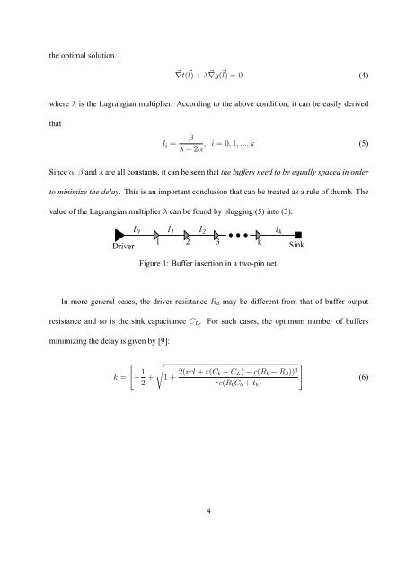
Since α, β and λ are all constants, it can be seen that the buffers need to be equally spaced in order
to minimize the delay. This is an important conclusion that can be treated as a rule of thumb. The
value of the Lagrangian multiplier λ can be found by plugging (5) into (3).
Driver
l
l l l
2 3 k
0 1 2 k
1
Sink
Figure 1: Buffer insertion in a two-pin net.
In more general cases, the driver resistance R d may be different from that of buffer output
resistance and so is the sink capacitance C L . For such cases, the optimum number of buffers
minimizing the delay is given by [9]:
k =
⌊− 1 2 + √
1 + 2(rcl + r(C b − C L ) − c(R b − R d )) 2
rc(R b C b + t b )
⌋
(6)
4