Buffer Insertion Basics - Computer Engineering & Systems Group ...

v
R min
v 2
v 3 ... v k
v 1
T(v 1
)
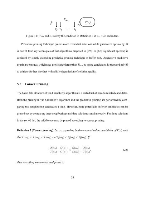
Figure 14: If α 1 and α 2 satisfy the condition in Definition 1 at v 1 , α 2 is redundant.
Predictive pruning technique prunes more redundant solutions while guarantees optimality. It
is one of four key techniques of fast algorithms proposed in [39]. In [42], significant speedup is
achieved by simply extending predictive pruning technique to buffer cost. Aggressive predictive
pruning technique, which uses a resistance larger than R min to prune candidates, is proposed in [43]
to achieve further speedup with a little degradation of solution quality.
5.3 Convex Pruning
The basic data structure of van Ginneken’s algorithms is a sorted list of non-dominated candidates.
Both the pruning in van Ginneken’s algorithm and the predictive pruning are performed by comparing
two neighboring candidates a time. However, more potentially inferior candidates can be
pruned out by comparing three neighboring candidate solutions simultaneously. For three solutions
in the sorted list, the middle one may be pruned according to convex pruning.
Definition 2 (Convex pruning) Let α 1 ,α 2 and α 3 be three nonredundant candidates of T(v) such
that C(α 1 ) < C(α 2 ) < C(α 3 ) and Q(α 1 ) < Q(α 2 ) < Q(α 3 ). If
Q(α 2 ) − Q(α 1 )
C(α 2 ) − C(α 1 ) < Q(α 3) − Q(α 2 )
C(α 3 ) − C(α 2 ) , (25)
then we call α 2 non-convex, and prune it.
33