Porosity Aware Buffered Steiner Tree Construction - Computer ...

More documents

Recommendations

Info

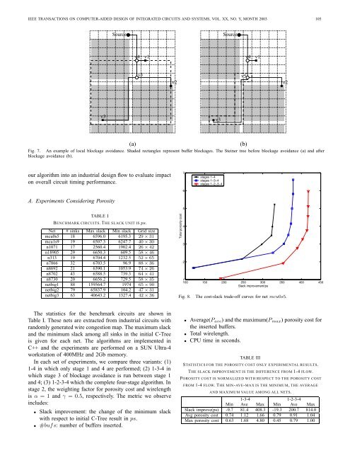
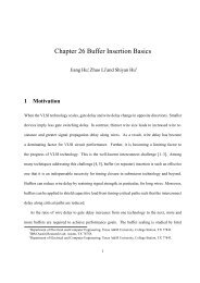
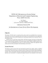
IEEE TRANSACTIONS ON COMPUTER-AIDED DESIGN OF INTEGRATED CIRCUITS AND SYSTEMS, VOL. XX, NO. Y, MONTH 2003 105SourceSourcev4v1v4v1v5v2v5v2v3v3(a)(b)Fig. 7. An example of local blockage avoidance. Shaded rectangles represent buffer blockages. The Steiner tree before blockage avoidance (a) and afterblockage avoidance (b).our algorithm into an industrial design flow to evaluate impacton overall circuit timing performance.A. Experiments Considering Porosity76stages 1−4stages 1−3−4stages 1−2−3−4TABLE IBENCHMARK CIRCUITS.THE SLACK UNIT IS ps.Net # sinks Max slack Min slack Grid sizemcu0s5 18 6596.0 6195.3 29 × 31mcu1s9 19 6507.3 6247.7 40 × 30n1071 17 2560.4 1902.4 26 × 42n18905 29 6650.3 609.5 58 × 46n313 19 6704.4 1232.5 52 × 65n7866 32 6703.5 96.9 88 × 36n8692 21 6390.1 1053.9 74 × 26n8702 43 6588.5 739.3 64 × 41n8730 20 6656.2 729.5 58 × 35netbig1 88 159564.7 1974 65 × 90netbig2 79 65837.9 104.2 47 × 31netbig3 63 40643.2 1327.4 42 × 36Total porosity cost54321100 150 200 250 300 350 400 450Slack improvement/psFig. 8.The cost-slack trade-off curves for net mcu0s5.The statistics for the benchmark circuits are shown inTable I. These nets are extracted from industrial circuits withrandomly generated wire congestion map. The maximum slackand the minimum slack among all sinks in the initial C-Treeis given for each net. The algorithms are implemented inC++ and the experiments are performed on a SUN Ultra-4workstation of 400MHz and 2Gb memory.In each set of experiments, we compare three variants: (1)1-4 in which only stage 1 and 4 are performed; (2) 1-3-4 inwhich stage 3 of blockage avoidance is run between stage 1and 4; (3) 1-2-3-4 which the complete four-stage algorithm. Instage 2, the weighting factor for porosity cost and wirelengthis α =1and γ =0.5, respectively. The metric we observeincludes:• Slack improvement: the change of the minimum slackwith respect to initial C-Tree result in ps.• #bufs: number of buffers inserted.• Average(P ave ) and the maximum(P max ) porosity cost forthe inserted buffers.• Total wirelength.• CPU time in seconds.TABLE IIISTATISTICS FOR THE POROSITY COST ONLY EXPERIMENTAL RESULTS.THE SLACK IMPROVEMENT IS THE DIFFERENCE FROM 1-4 FLOW.POROSITY COST IS NORMALIZED WITH RESPECT TO THE POROSITY COSTFROM 1-4 FLOW. THE MIN-AVE-MAX IS THE MINIMUM, THE AVERAGEAND MAXIMUM VALUE AMONG ALL NETS.1-3-4 1-2-3-4Min Ave Max Min Ave MaxSlack improve(ps) -9.7 81.4 408.3 -19.3 200.7 814.0Avg porosity cost 0.74 1.12 1.66 0.79 0.91 1.04Max porosity cost 0.63 1.68 4.80 0.45 0.79 1.00
IEEE TRANSACTIONS ON COMPUTER-AIDED DESIGN OF INTEGRATED CIRCUITS AND SYSTEMS, VOL. XX, NO. Y, MONTH 2003 106TABLE IIEXPERIMENTAL RESULTS WHEN ONLY POROSITY COST IS MINIMIZED.POROSITY COST IS DENOTED AS P .Net Flow Slack impr P ave #buf P max Wirelen CPU(s)1-4 330.80 0.75 7 1.25 10830 0.91mcu0s5 1-3-4 378.58 0.73 9 1.16 10830 3.751-2-3-4 417.97 0.66 9 0.85 12513 8.821-4 865.50 0.57 12 1.02 12600 4.60mcu1s9 1-3-4 876.40 0.52 13 0.64 12600 17.361-2-3-4 911.90 0.50 14 0.50 13726 74.411-4 126.02 2.56 2 2.56 3837 0.10n1071 1-3-4 189.23 1.90 4 2.56 3837 0.391-2-3-4 203.21 2.03 5 2.56 3997 4.661-4 1927.62 0.60 9 1.38 16461 2.63n18905 1-3-4 1964.95 0.94 12 3.25 16461 5.641-2-3-4 2230.13 0.51 14 0.61 18999 23.171-4 382.02 1.89 5 2.09 16245 0.22n313 1-3-4 386.39 1.94 9 2.09 16245 1.951-2-3-4 452.01 1.65 10 2.09 17555 11.571-4 2332.62 1.05 5 1.67 16617 0.82n7866 1-3-4 2358.14 0.94 3 1.67 16617 23.981-2-3-4 2365.44 0.94 3 1.67 16379 61.651-4 1912.96 0.55 19 1.02 13929 149.33n8692 1-3-4 1907.25 0.72 23 3.28 14373 67.921-2-3-4 1893.71 0.52 21 0.90 14978 83.241-4 4322.21 2.09 9 3.42 14496 1.07n8702 1-3-4 4430.78 2.12 14 3.42 14202 25.361-2-3-4 4599.57 1.80 19 2.40 14967 89.141-4 1760.20 0.62 11 1.84 15363 3.52n8730 1-3-4 1830.23 0.73 14 3.69 15363 9.291-2-3-4 1945.03 0.60 17 1.06 17211 22.381-4 6209.30 0.58 28 1.67 59004 35.67netbig1 1-3-4 6436.58 0.70 38 3.11 59004 39.571-2-3-4 6653.41 0.60 40 1.46 64830 79.101-4 873.35 2.18 8 2.76 44106 0.74netbig2 1-3-4 1281.61 2.40 16 2.76 44106 3.251-2-3-4 1687.39 2.12 23 2.76 48911 30.791-4 330.23 1.54 2 1.67 29370 0.81netbig3 1-3-4 401.03 1.59 3 1.67 29370 1.091-2-3-4 552.99 1.45 7 1.67 31115 17.71The results for set 1 are shown in Table II with its statisticsin Table III. The data in Table III show that the complete1-2-3-4 flow can achieve 200ps slack improvement over 1-4 flow and 120ps improvement over 1-3-4 flow on average.The average porosity cost P ave is an average value for allbuffers inserted in a net and P max is the maximum porosityamong all buffers. The average porosity cost is reduced by 9%from 1-4 flow. Since 1-3-4 flow does not consider porosity, itsrerouting in stage 3 increases the average porosity cost by12%. The effect is more significant for the maximum porositycost P max . The 1-2-3-4 flow achieves 21% maximum porositycost reduction while the 1-3-4 flow results in 68% greatercost. Therefore, the stage 2 is very necessary on improvingboth timing and porosity cost. In order to further illustratethe effect of our algorithm, the cost-slack trade-off curves ofnet mcu0s5 for different flows are shown in Figure 8. Thesecurves come from the final candidate solutions at the rootnode in Van Ginneken’s algorithm at stage 4. Obviously, thesolutions from our proposed 1-2-3-4 flow is better on bothtiming and cost. The CPU time is concluded in the rightmostcolumn of Table II.B. Experiments Considering Wiring CongestionWe also tested the effect of our algorithm on wiring congestionfor the same set of testcases in Section IV-A. Whenwiring congestion is considered, only the cost function in stage2 is changed by augmenting wire density cost βd 2 where dis the wire density. Average(D ave ) and the maximum(D max )wire density over all tile boundaries the edges of the Steinertree crossing are reported in the experimental results.Table IV and Table V show results from experiments inwhich wire density is considered but porosity cost is ignored.In these experiments, the weighting factors for porosity cost,wire density and scaled wirelength are α = 0,β = 1 andγ =0.25, respectively. The statistics in Table V shows thatthe average wire density, which is the average of the wiredensity among all the tile boundaries the routing tree across,is improved by 30%. The peak wire density is reduced by 19%as well.The combination of porosity and wiring congestion is testedand the results are listed in Table VI and Table VII. In theseexperiments, the weighting factors for porosity cost, wiredensity and scaled wirelength are α =1,β =0.5 and γ =0.1,respectively. Since the only different part is in stage 2, theresults of flow 1 − 4 and flow 1 − 3 − 4 are the same as thosein Table II and Table IV. However, the statistics for flow 1-3-4is shown in Table VII for the ease of comparison. Sometimeswire density is increased by our algorithm. However, thisnormally happens when the wire density of the initial C-Treeis low. For example, the average wire density is increased from
Page 1 and 2: IEEE TRANSACTIONS ON COMPUTER-AIDED
Page 5: IEEE TRANSACTIONS ON COMPUTER-AIDED

Porosity Aware Buffered Steiner Tree Construction - Computer ...

You also want an ePaper? Increase the reach of your titles

Delete template?

Save as template?