Liquid interfaces in viscous straining flows ... - Itai Cohen Group

More documents

Recommendations

Info

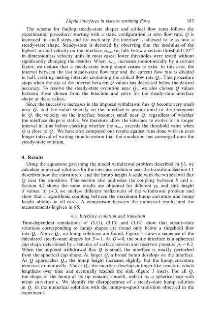
Liquid interfaces in viscous straining flows 183The scheme for finding steady-state shapes and critical flow rates follows theexperimental procedure: starting with a static configuration at zero flow rate, Q isincreased in small steps and for each step the interface is allowed to relax into asteady-state shape. Steady-state is detected by observing that the modulus of thehighest normal velocity on the interface, u max · n, falls below a certain threshold (10 −3in dimensionless velocity units in most cases; lower thresholds were tested withoutsignificantly changing the results). When u max increases monotonically by a certainfactor, we deduce that a steady-state hump shape ceases to exist. In this case, theinterval between the last steady-state flow rate and the current flow rate is dividedin half, creating nesting intervals containing the critical flow rate Q c . This procedurestops when the size of the interval between Q values has decreased below the desiredaccuracy. To resolve the steady-state evolution near Q c ,wealsochooseQ valuesbetween those chosen from the bisection and solve for the steady-state interfaceshape at these values.Since the successive increases in the imposed withdrawal flux Q become very smallnear Q c and the initial velocity on the interface is proportional to the incrementin Q, the velocity on the interface becomes small near Q c regardless of whetherthe interface shape is stable. We therefore allow the interface to evolve for a longerinterval in time before checking whether the u max exceeds the threshold value whenQ is close to Q c . We have also compared our results against runs done with an evenlonger interval of waiting time to ensure that the simulation has converged onto thesteady-state solution.4. ResultsUsing the equations governing the model withdrawal problem described in § 3, wecalculate numerical solutions for the interface evolution near the transition. Section 4.1describes how the curvature κ and the hump height h scale with the withdrawal fluxQ near the transition. This section also addresses the coupling between h and κ.Section 4.2 shows the same results are obtained for different p 0 and sink heightS values. In § 4.3, we analyse different realizations of the withdrawal problem andshow that a logarithmic coupling between the maximum hump curvature and humpheight obtains in all cases. A comparison between the numerical results and themeasurements is given in § 5.4.1. Interface evolution and transitionTime-dependent simulations of (3.11), (3.13) and (3.14) show that steady-statesolutions corresponding to hump shapes are found only below a threshold flowrate Q c .AboveQ c , no hump solutions are found. Figure 3 shows a sequence of thecalculated steady-state shapes for S =1. At Q = 0, the static interface is a sphericalcap shape determined by a balance of surface tension and reservoir pressure p 0 =0.2.When the imposed withdrawal flux Q is small, the interface is weakly perturbedfrom the spherical cap shape. At larger Q, a broad hump develops on the interface.As Q approaches Q c , the hump height increases slightly, but the hump curvatureincreases dramatically. Above Q c , the interface develops a finger-like structure whichlengthens over time and eventually reaches the sink (figure 3 inset). For all Q,the shape of the hump at its tip remains smooth, well-fit by a spherical cap withmean curvature κ. We identify the disappearance of a steady-state hump solutionat Q c in the numerical solutions with the hump-to-spout transition observed in theexperiment.
184 M. Kleine Berkenbusch, I. Cohen and W. W. ZhangQ cStrong flowQ = 0Figure 3. Steady-state interface shapes (solid lines) at different Q. ForQ = 0, the interfaceassumes a spherical cap shape for which the Laplace pressure balances the reservoir pressurep 0 .AsQ increases, the steady-state shape develops a hump towards the sink. The inset showsthat, above the transition withdrawal flux Q c , the unsteady interface (dashed line) developsa finger reaching towards the sink. Here, the dimensionless sink height S ≡ ˜S/a =1 and thedimensionless reservoir pressure jump p 0 is 0.2.In the rest of this subsection, we will analyse a typical set of results, obtainedwith dimensionless sink height S =0.2 and reservoir pressure p 0 set to 0.01. We canquantitatively characterize the interface evolution by plotting the hump height h andthe mean curvature κ at the tip of the hump as functions of the withdrawal flux Q(figure 4). As Q approaches Q c , the hump height saturates at h c (figure 4a) and thecurvature saturates at κ c (figure 4b). The insets show that h and κ approach theirsaturation values ash c − h∝ √ δq,h cκ c − κκ c∝ √ δq, δq ≡ Q c − QQ c. (4.1)To obtain the best power-law fit, the h c and Q c values were adjusted slightly. Thebest fit is obtained when the values of h c and Q c were increased from the h and Qvalues corresponding to the final steady-state hump shape calculated by 0.03 % and4 × 10 −5 %, respectively. The κ c value is adjusted by less than 0.001 % from the finalhump curvature value obtained numerically. The same Q c value is used in all theplots. All the adjustments are within the error bars of the simulation.The observed square-root dependence of h c − h and κ c − κ suggests that thetransition from selective withdrawal to viscous entrainment occurs via a collision atQ c of two steady-state hump solutions, one stable and one unstable. In other words,the transition from selective withdrawal to viscous withdrawal has the structureof a saddle-node bifurcation. Typically, saddle-node bifurcations are associated withsolutions that remain smooth at the bifurcation point. Therefore, the observed squarerootscaling suggests that the final evolution of the interface as the transition isapproached is not organized by an approach towards a singular steady-state shape.The saddle-node structure of the transition can be rationalized by considering theflow in the upper layer. It converges along the centreline and therefore speeds up awayfrom the tip of the hump. Since the hump solution is realized in a time-dependentsimulation and also observed in the experiment, it is linearly stable. We thereforeexpect that small upwards, perturbations of the hump tip simply decay downwardsas the hump shape relaxes towards the steady-state solution over time. However,if the upwards perturbation is very large, so that the perturbed hump tip now liesvery close to the sink, then surface tension effects will be too weak to pull theperturbed interface downwards. Instead, the hump tip will be drawn into the sink.
Page 6 and 7: Liquid interfaces in viscous strain
Page 26 and 27: 10 0Liquid interfaces in viscous st
Page 34: Liquid interfaces in viscous strain

Liquid interfaces in viscous straining flows ... - Itai Cohen Group

Create successful ePaper yourself

Delete template?

Save as template?