Liquid interfaces in viscous straining flows ... - Itai Cohen Group

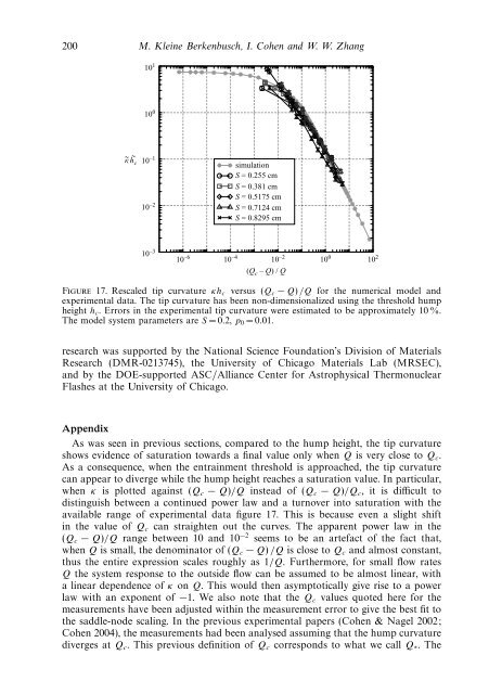
200 M. Kleine Berkenbusch, I. Cohen and W. W. Zhang~ h~ c10 110 010 –1simulationS = 0.255 cmS = 0.381 cmS = 0.5175 cm10 –2S = 0.7124 cmS = 0.8295 cm10 –310 –6 10 –4 10 –2 10 0 10 2(Q c – Q) / QFigure 17. Rescaled tip curvature κh c versus (Q c − Q) /Q for the numerical model andexperimental data. The tip curvature has been non-dimensionalized using the threshold humpheight h c . Errors in the experimental tip curvature were estimated to be approximately 10 %.The model system parameters are S =0.2, p 0 =0.01.research was supported by the National Science Foundation’s Division of MaterialsResearch (DMR-0213745), the University of Chicago Materials Lab (MRSEC),and by the DOE-supported ASC/Alliance Center for Astrophysical ThermonuclearFlashes at the University of Chicago.AppendixAs was seen in previous sections, compared to the hump height, the tip curvatureshows evidence of saturation towards a final value only when Q is very close to Q c .As a consequence, when the entrainment threshold is approached, the tip curvaturecan appear to diverge while the hump height reaches a saturation value. In particular,when κ is plotted against (Q c − Q)/Q instead of (Q c − Q)/Q c , it is difficult todistinguish between a continued power law and a turnover into saturation with theavailable range of experimental data figure 17. This is because even a slight shiftin the value of Q c can straighten out the curves. The apparent power law in the(Q c − Q)/Q range between 10 and 10 −2 seems to be an artefact of the fact that,when Q is small, the denominator of (Q c − Q) /Q is close to Q c and almost constant,thus the entire expression scales roughly as 1/Q. Furthermore, for small flow ratesQ the system response to the outside flow can be assumed to be almost linear, witha linear dependence of κ on Q. This would then asymptotically give rise to a powerlaw with an exponent of −1. We also note that the Q c values quoted here for themeasurements have been adjusted within the measurement error to give the best fit tothe saddle-node scaling. In the previous experimental papers (Cohen & Nagel 2002;Cohen 2004), the measurements had been analysed assuming that the hump curvaturediverges at Q c . This previous definition of Q c corresponds to what we call Q ∗ .The