Liquid interfaces in viscous straining flows ... - Itai Cohen Group

More documents

Recommendations

Info

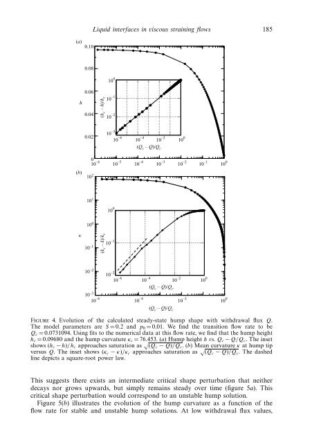
Liquid interfaces in viscous straining flows 185(a)0.100.08h0.060.04(h c – h)/h c10 010 –110 –210 –5 10 –4(b)0.0210 –310 –6010 –610 210 –4 10 –2 10 0(Q c – Q)/Q c10 –3 10 –2 10 –1 10 010 110 010 0κ10 –1(k c – k)/k c10 010 –210 –210 –6 10 –4 10 –210 –1 (Q c – Q)/Q c10 –310 –6 10 –4 10 –2 10 0(Q c – Q)/Q cFigure 4. Evolution of the calculated steady-state hump shape with withdrawal flux Q.The model parameters are S =0.2 and p 0 =0.01. We find the transition flow rate to beQ c =0.0731094. Using fits to the numerical data at this flow rate, we find that the hump heighth c =0.09680 and the hump curvature κ c =76.453. (a) Humpheighth vs. Q c − Q/Q c . The insetshows (h c − h)/h c approaches saturation as √ (Q c − Q)/Q c .(b) Mean curvature κ at hump tipversus Q. The inset shows (κ c − κ)/κ c approaches saturation as √ (Q c − Q)/Q c . The dashedline depicts a square-root power law.This suggests there exists an intermediate critical shape perturbation that neitherdecays nor grows upwards, but simply remains steady over time (figure 5a). Thiscritical shape perturbation would correspond to an unstable hump solution.Figure 5(b) illustrates the evolution of the hump curvature as a function of theflow rate for stable and unstable hump solutions. At low withdrawal flux values,
186 M. Kleine Berkenbusch, I. Cohen and W. W. Zhang(a)(b)κUnstable humpUnstable steady state solutionκ cStable humpNo hump solutionStable steady state solutionQ cQFigure 5. (a) Stable and unstable hump solutions in steady-state selective withdrawal. (b)Saddle-node bifurcation diagram illustrating the evolution of the hump curvature in thenselective withdrawal regime.only a very large shape perturbation can cause the interface to be drawn into thesink, we therefore expect the stable and the unstable hump shapes to be widelyseparated. This means the unstable hump must lie close to the sink and, as a result,has a very curved tip. At moderate withdrawal flux values, the perturbation sizerequired to destabilize the hump solution becomes smaller, implying that the unstableand stable solutions now lie closer to each other. Concurrently, the curvature of thestable solution increases, and the curvature of the unstable solution decreases. Neartransition, even a small perturbation causes the interface to become unstable andgrow towards the sink. This suggests the two solutions lie very close each other andare nearly identical. Therefore it is reasonable to expect the two solutions to becomeidentical, or coincide, at Q c , thereby bringing about a saddle-node bifurcation of thehump solution. The square-root scaling corresponds to a smooth merging of the twosolutions, so that the κ(Q) curve at Q c has the shape of a parabola lying on its side.The scaling dynamics associated with how the hump solution saturates as Qapproaches Q c is consistent with a saddle-node bifurcation at Q c .Thisisagenericmechanism for transition to one type of solution from another in a dynamicalsystem with only a few degrees of freedom and suggests that the dynamics of theentire interface is coupled. However, the quantitative analysis in figure 4 shows anatypical feature: the hump height and curvature saturate towards the final scalingbehaviour at very different δq values. Specifically, the square-root scaling in h c − his evident throughout its evolution, even at large δq. In contrast, the square-rootscaling for κ c − κ becomes evident only when δq has decreased below 10 −3 .Thisbehaviour suggests the hump shape does not approach the transition uniformly. Totest this idea, we plot the hump radius at z = h/2 as a function of Q (figure 6). Wefind that the radius at the half-height saturates to the final scaling behaviour laterthan h, but earlier than κ as δq approaches 0. This behaviour indicates that, as Qapproaches Q c , the overall shape of the hump, e.g. the hump height or its lateral extent,saturates first, followed by features on smaller length scales. The shape of the hump atits tip, which corresponds to a feature on the smallest length scale, saturates last. Thiscascade of events is more typical of an approach towards a singular shape, in whichfeatures evolving on different length scales are nearly decoupled, so that features onsmaller length scales saturate later than features on large length scales.To obtain some insight into this unusual hybrid character of the interface evolutionnear transition, we plot κ as a function of h (figure 7). At Q = 0, the interface shape
Page 6 and 7: Liquid interfaces in viscous strain
Page 26 and 27: 10 0Liquid interfaces in viscous st
Page 34: Liquid interfaces in viscous strain

Liquid interfaces in viscous straining flows ... - Itai Cohen Group

You also want an ePaper? Increase the reach of your titles

Delete template?

Save as template?