Liquid interfaces in viscous straining flows ... - Itai Cohen Group

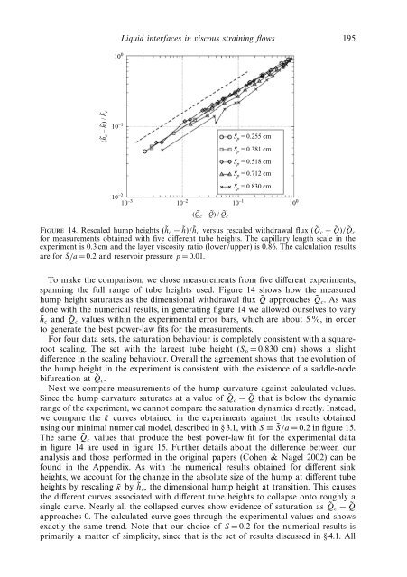
10 0Liquid interfaces in viscous straining flows 195(h ~ c – h~ ) / h ~ c10 –1S p = 0.255 cmS p = 0.381 cmS p = 0.518 cmS p = 0.712 cmS p = 0.830 cm10 –2 10 –3 10 –2 (Q ~ c – Q~ ) / Q ~ c10 –1 10 0Figure 14. Rescaled hump heights (˜h c − ˜h)/˜h c versus rescaled withdrawal flux ( ˜Q c − ˜Q)/ ˜Q cfor measurements obtained with five different tube heights. The capillary length scale in theexperiment is 0.3 cm and the layer viscosity ratio (lower/upper) is 0.86. The calculation resultsare for ˜S/a =0.2 and reservoir pressure p =0.01.To make the comparison, we chose measurements from five different experiments,spanning the full range of tube heights used. Figure 14 shows how the measuredhump height saturates as the dimensional withdrawal flux ˜Q approaches ˜Q c .Aswasdone with the numerical results, in generating figure 14 we allowed ourselves to vary˜h c and ˜Q c values within the experimental error bars, which are about 5 %, in orderto generate the best power-law fits for the measurements.For four data sets, the saturation behaviour is completely consistent with a squarerootscaling. The set with the largest tube height (S p =0.830 cm) shows a slightdifference in the scaling behaviour. Overall the agreement shows that the evolution ofthe hump height in the experiment is consistent with the existence of a saddle-nodebifurcation at ˜Q c .Next we compare measurements of the hump curvature against calculated values.Since the hump curvature saturates at a value of ˜Q c − ˜Q that is below the dynamicrange of the experiment, we cannot compare the saturation dynamics directly. Instead,we compare the ˜κ curves obtained in the experiments against the results obtainedusing our minimal numerical model, described in § 3.1, with S ≡ ˜S/a =0.2 in figure 15.The same ˜Q c values that produce the best power-law fit for the experimental datain figure 14 are used in figure 15. Further details about the difference between ouranalysis and those performed in the original papers (Cohen & Nagel 2002) can befound in the Appendix. As with the numerical results obtained for different sinkheights, we account for the change in the absolute size of the hump at different tubeheights by rescaling ˜κ by ˜h c , the dimensional hump height at transition. This causesthe different curves associated with different tube heights to collapse onto roughly asingle curve. Nearly all the collapsed curves show evidence of saturation as ˜Q c − ˜Qapproaches 0. The calculated curve goes through the experimental values and showsexactly the same trend. Note that our choice of S =0.2 for the numerical results isprimarily a matter of simplicity, since that is the set of results discussed in § 4.1. All