Liquid interfaces in viscous straining flows ... - Itai Cohen Group

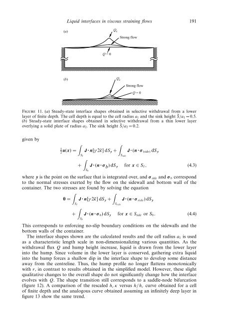
Liquid interfaces in viscous straining flows 191(a)Q cStrong flowQ = 0(b)Q cStrong flowQ = 0Figure 11. (a) Steady-state interface shapes obtained in selective withdrawal from a lowerlayer of finite depth. The cell depth is equal to the cell radius a 1 and the sink height ˜S/a 1 =0.5.(b) Steady-state interface shapes obtained in selective withdrawal from a thin lower layeroverlying a solid plate of radius a 2 . The sink height ˜S/a 2 =0.2.given by∫1u(x) = J · n[γ 2˜κ]dS2 y + J · (n · σ (side) dS y∫S I S side∫+ J · (n · σ b )dS y for x ∈ S I , (4.3)S bwhere y is the point on the surface that is integrated over, and σ side and σ b correspondto the normal stresses exerted by the flow on the sidewall and bottom wall of thecontainer. The two stresses are found by solving the equation∫∫0 = J · n[γ 2˜κ]dS y + J · (n · σ side )dS yS I S side∫+ J · (n · σ b )dS y for x ∈ S side or S b . (4.4)S bThis corresponds to enforcing no-slip boundary conditions on the sidewalls and thebottom walls of the container.The interface shapes shown are the calculated results and the cell radius a 1 is usedas a characteristic length scale in non-dimensionalizing various quantities. As thewithdrawal flux Q and hump height increase, liquid is drawn from the lower layerinto the hump. Since volume in the lower layer is conserved, gathering extra liquidinto the hump forces a shallow dip in the interface shape to develop some distanceaway from the centreline. Thus, the hump profile no longer flattens monotonicallywith r, in contrast to results obtained in the simplified model. However, these slightqualitative changes to the overall shape do not significantly change how the interfaceevolves with Q. The shape transition still corresponds to a saddle-node bifurcation(figure 12). A comparison of the rescaled h c κ versus h/h c curve obtained for a cellof finite depth and the analogous curve obtained assuming an infinitely deep layer infigure 13 show the same trend.