Car Ownership? Evidence from the Copenhagen Metropolitan Area

Recommendations

Info

∑ ∑ ∑ ,, , which implies that the choice probabilities are given by the multinomial logit model (MNL). 9 We are interested in what the model can tell us about the decision to own a car and the impact public transport has on that decision. The consumer will own a car if the maximum utility of the alternatives in which a car is owned exceeds the maximum utility of the alternatives in which no car is owned. The former maximum utility, which we denote as ,, | 1 is: ln∑ ∑ ,, . (3) For the utility U of not having a car we have: ln∑ ∑ ,, . (4) The first terms on the right-hand side of (3) and (4) are known as the logsums. The random terms and are independent and Extreme Value Type I distributed. The choice whether or not to own a car can therefore be described as a binomial logit model in which the logsums are the deterministic parts of the utilities. Denoting the probability of car ownership as we thus have: ∑ ∑ ,, ∑ ∑ ,, ∑ ∑ ,, (5) It should be noted that this model differs from one in which we estimate car ownership conditional on the choice of a residential area and housing type, as is the case in the literature on the impact of urban form on car ownership cited in the introduction. In that literature binomial models of the type: |, ,, ,, (6) ,, 9 That is: ,, ,, ∑ ∑ ∑ ,, . 10
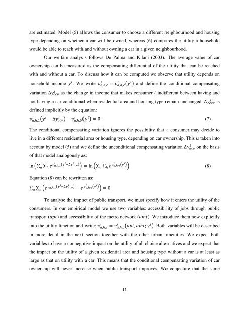
are estimated. Model (5) allows the consumer to choose a different neighbourhood and housing type depending on whether a car will be owned, whereas (6) compares the utility a household would be able to reach with and without owning a car in a given neighbourhood. Our welfare analysis follows De Palma and Kilani (2003). The average value of car ownership can be measured as the compensating differential of the utility that can be reached with and without a car. To discuss how it can be computed we observe that utility depends on household income . We write ,, ,, and define the conditional compensating variation ∆ as the change in income that makes consumer indifferent between having and not having a car conditional when residential area and housing type remain unchanged. ∆ is defined implicitly by the equation: ,, ∆ ,, 0 . (7) The conditional compensating variation ignores the possibility that a consumer may decide to live in a different residential area or housing type, depending on car ownership. This is taken into account by model (5) and we define the unconditional compensating variation ∆ on the basis of that model analogously as: ln ∑ ∑ ,, ∆ Equation (8) can be rewritten as: ∑ ∑ ,, ∆ ln∑ ∑ ,, (8) ,, 0 To analyse the impact of public transport, we must specify how it enters the utility of the consumers. In our empirical model we use two variables: accessibility of jobs through public transport () and accessibility of the metro network (). We introduce them now explicitly into the utility function and write: ,, ,, , ; . Both variables will be described in more detail in the next section together with the other urban amenities. We expect both variables to have a nonnegative impact on the utility of all choice alternatives and we expect that the impact on the utility of a given residential area and housing type without a car is at least as large as that on utility with a car. This means that the conditional compensating variation of car ownership will never increase when public transport improves. We conjecture that the same 11
Page 1 and 2: TI 2015-139/VIII Tinbergen Institut
Page 3: Does improving public transport dec
Page 6 and 7: even in transportation the impact o
Page 8 and 9: It is a fair simplification to clai
Page 10 and 11: of owner-occupied residences consti
Page 12 and 13: 3. The model This section presents
Page 16 and 17: holds for the unconditional compens
Page 18 and 19: sum of the average utility of the a
Page 20 and 21: characteristics that make an area a
Page 22 and 23: the last six are characterizing the
Page 24 and 25: determined by the demographic compo
Page 26 and 27: second stage we put the estimated v
Page 28 and 29: Table 4.a First step estimation pro
Page 30 and 31: preferred to apartments and a highe
Page 32 and 33: Map 5. Metro system extension 6.1.
Page 34 and 35: Map 7. Change in relative house pri
Page 36 and 37: demographic composition of neighbou
Page 38 and 39: Table 6: Compensating variations of
Page 40 and 41: area. Since it is difficult to choo
Page 42 and 43: Judd, K. 1998. Numerical Methods in
Page 44 and 45: Table A.1.2. Hedonic price equation
Page 46 and 47: Table A.2.2 First step IV estimatio
Page 48 and 49: Map A.2. Pct. change in population
Page 50 and 51: Map A.4. Pct. change in the share o
Page 52 and 53: Map A.6. Pct. change in the number
Page 54 and 55: In this equation the levels of ,

Car Ownership? Evidence from the Copenhagen Metropolitan Area

Create successful ePaper yourself

Delete template?

Save as template?