MATLAB by rudra pratap

6.1 Basic 2-D Plots
181
Method 3: Using the line command to generate overlay plots
The line is a low-level graphics command used by the plot command to generate
lines. Once a plot exists in the graphics window, additional lines may be added by
using the line command directly. The line command takes a pair of vectors (or a
triplet in 3-D) followed by parameter name/parameter· value pairs as arguments:
line (xdata, ydata, ParameterName, ParameterVaLue)
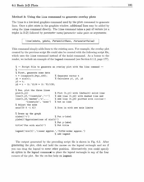
This command simply adds lines to the existing axes. For example, the overlay plot
created by the previous script file could also be created with the following script file,
which uses the line command instead of the hold command. As a bonus to the
reader, we include an example of the legend command (see Section 6.1.2, page 177).
% -- Script file to generate an overlay plot Yith the line command --
% ------------------
% First , generate some data
t = linspace (0 , 2*pi,100) ; % Generate vector t
yl sin(t) ;
% Calculate yl , y2 , y3
y2 t;
y3 t - (t . -3)/6 + (t . 5)/120;
% NoY , plot the three lines
plot (t ,y1)
line (t, y2 , 'linestyle ' ,'-- ')
line(t,y3, 'marker ' , 'o' , ...
'linestyle ', 'none ')
% Adjust the axes
axis([O 5 -1 5] )
% Plot (t ,y1) Yith (default) solid line
% Add line (t ,y2) with dashed line and
% Add line (t ,y3) plotted with circles-­
% but no line
% Zoom in with new ax is limits
% Dress up the graph
xlabel ('t')
% Put x-label
ylabel ('Approximat ions of sin(t) ')
% Put y-label
title ('Fun with sin(t) ') % Put title
legend('sin(t) ' ,'linear approx . ' ,'fifth-order approx .')
% add legend
The output generated by the preceding script file is shown in Fig. 6.3. After
generating the plot, click and hold Lhe mouse on the legend rect angle a.mi Bcc if
you can drag the legend to some other position. Alternatively, you could specify
an option in the legend command to place the legen