SAS/STAT 922 User's Guide: The MIXED Procedure (Book Excerpt)

4556 ✦ Chapter 56: The MIXED Procedure
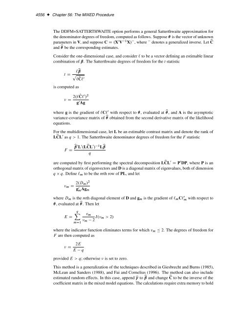
The DDFM=SATTERTHWAITE option performs a general Satterthwaite approximation for
the denominator degrees of freedom, computed as follows. Suppose is the vector of unknown
parameters in V, and suppose C D .X 0 V 1 X/ , where denotes a generalized inverse. Let bC
and b be the corresponding estimates.
Consider the one-dimensional case, and consider ` to be a vector defining an estimable linear
combination of ˇ. The Satterthwaite degrees of freedom for the t statistic
t D `bˇ
p
` OC` 0
is computed as
D 2.` OC` 0 / 2
g 0 Ag
where g is the gradient of `C` 0 with respect to , evaluated at b, and A is the asymptotic
variance-covariance matrix of b obtained from the second derivative matrix of the likelihood
equations.
For the multidimensional case, let L be an estimable contrast matrix and denote the rank of
LbCL 0 as q > 1. The Satterthwaite denominator degrees of freedom for the F statistic
F D bˇ 0 L 0 .LbCL 0 / 1 Lbˇ
q
are computed by first performing the spectral decomposition LbCL 0 D P 0 DP, where P is an
orthogonal matrix of eigenvectors and D is a diagonal matrix of eigenvalues, both of dimension
q q. Define `m to be the mth row of PL, and let
m D
2.Dm/ 2
g 0 m Agm
where Dm is the mth diagonal element of D and gm is the gradient of `mC` 0 m
, evaluated at b. Then let
E D
qX
mD1
m
m
2 I. m > 2/
where the indicator function eliminates terms for which m
F are then computed as
D 2E
E q
provided E > q; otherwise is set to zero.
with respect to
2. The degrees of freedom for
This method is a generalization of the techniques described in Giesbrecht and Burns (1985),
McLean and Sanders (1988), and Fai and Cornelius (1996). The method can also include
estimated random effects. In this case, append b to bˇ and change bC to be the inverse of the
coefficient matrix in the mixed model equations. The calculations require extra memory to hold