Tracking Ocean Wanders (PDF, 5 MB) - BirdLife International

Tracking ocean wanderers: the global distribution of albatrosses and petrels – Methods
2.4 METHODS FOR ANALYSING GLS DATA
Geolocation (Global Location Sensing or GLS-logging) is
an alternative to satellite-telemetry for determining animal
location. GLS loggers record light levels and use the timing
of local noon and midnight to estimate longitude, and day
length to estimate latitude. Although not as accurate as
satellite tags, their small size and longevity mean that they
are ideally suited to long-term deployment, and are
therefore highly effective for migration studies.
The GLS technique provides 2 locations per day (at
local midday and midnight) except for a variable period
around the equinox when it is impossible to estimate
latitude. The accuracy of the technique varies but given the
type of device, processing technique and study-species it is
reasonable to assume, based on data collected between 30°S
and 60°S, an average error of around 186 km for GLS
datasets submitted to the workshop (Phillips et al. 2004a).
2.4.1 Standardisation of GLS data
A variety of GLS loggers are available, differing in both
design and recording interval. Techniques for converting
light levels to location estimates also vary (e.g. threshold
methods compared with curve-fitting), as do approaches to
subsequent post-processing to remove unrealistic locations.
The latter is a particularly time-consuming part of the
analysis. For these reasons it was deemed unrealistic to
develop a standardised validation routine for the GLS
component of the workshop tracking data.
Data contributors were therefore asked to submit postprocessed
GLS locations and provide brief metadata on the
conversion methods and validation rules that had been
applied. In fact, there was little difference in the proportion
of points eliminated in each of the four GLS datasets
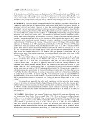
Table 2.2. Format of the standardised GLS tracking data.
submitted to the workshop (6.9%, 15.2%, 5.9% and 6.9% of
locations excluded during June and July and 21.0%, 22.8%,
24.5% and 29.6% of locations excluded in August).
The GLS tracking data were standardised according to
the format indicated in Table 2.2.
In order to separate breeding from non-breeding season
data, if individual-specific data were not provided, the
breeding season for a particular population was defined as
the time from the mean copulation date to mean fledging
date. All locations falling outside this date range were
assigned a status of N (non-breeder) and a stage of NB
(non-breeding).
2.4.2 Density distribution maps
As GLS locations are available from tracked birds at
approximately 12-hour intervals and invalid locations are
eliminated more or less randomly, there is no requirement to
resample the data. For a variable period around the
equinoxes, however, it is impossible to obtain location
estimates and consequently sample sizes were consistently
smaller during March and September and, to a lesser
extent, during April and August. Histograms presented
alongside each distribution map indicate the sample size
(bird days) per month, highlighting the underrepresentation
of ranges during certain periods.
The analysis of submitted GLS data was restricted to the
non-breeding period as (better quality) satellite-tracking
data were available for breeding birds for all species and sites
concerned. Kernel density distribution maps were generated
in ArcMap 8.1 using a smoothing factor of 2 degrees (the
nominal resolution of the GLS data) and a cell size of 0.5
degrees (see PTT methods section for further details).
Name Type Length Description
Species string 3 links to Species table
Site string 3 links to Site table
Colony string 3 links to Colony table, which in turn has linksto Site
TrackID string 10 unique track identifier, usually device ID + trip number, depending on what was provided
PointID integer sequential number to identify uplinks within a trip
DeviceID string 10 GLS identifier
DeviceType string 20 GLS device type
TripID integer sequential number to identify trips or stages within a deployment
BirdID string 10 ring number or other label to uniquely identify an individual
Age string 1 A: adult, J: subadult / juvenile / prebreeder, U: unknown
Sex string 1 M: male, F: female, U: unknown
Status string 1 B: breeder; N: non-breeder; U: unknown
Stage string 2 PE: pre-egg
IN: incubation
CK: chick (includes brood, guard and post-guard stages)
FM: failed breeder / migration after breeding
UN: unknown
Latitude float 8.4
Longitude float 8.4
DateGMT date
TimeGMT time
Code integer -9: invalidated by user
9: validated by user
Comments memo
Contributor memo
Reference memo
Janet Silk
9