Stave River Water Use Plan - BC Hydro

Stave River Water Use Plan: 

Monitoring Program Terms of Reference 

June 13, 2005 

BC Hydro Page 1

Stave River Water Use Plan 

Monitoring Terms of Reference June 13, 2005 

Overview 

Monitoring Program 

Stave River Water Use Plan: 

Monitoring Program Terms of Reference 

The Stave River Water Use Planning process was completed in the fall of 1999 

with the release of a consultative committee report (Failing 1999) and the submission of 

draft water use plan (WUP) to the provincial Comptroller of Water Rights. The water use 

planning process, which involved consultation with a committee of interested 

stakeholders to identify water use values and objectives, the completion of several 

ecological studies and a gaming procedure to develop balanced operational alternatives, 

resulted in substantial knowledge gains about the Stave lake watershed. Despite this 

considerable effort and the successful development of what the consultative committee 

(CC) considered to be a balanced WUP for the Stave Lake project (Combo 6 WUP 

operating strategy), a number of knowledge gaps and uncertainties remained. 

Conditional to the general acceptance the WUP by the CC was the development and 

implementation of monitoring program that addresses these shortcomings. 

At the conclusion of the WUP consultation process, the consultative committee 

(CC) were able identified three general areas of uncertainty. The first was the extent to 

which the productivity levels in both Stave and Hayward reservoirs would change when 

operations specified in the WUP are implemented. The productivity indicators of interest 

included seasonal nutrient levels, seasonal levels of photosynthetic carbon (an indicator 

of general lake productivity), seasonal levels of littoral periphyton production at various 

water depths, and a general assessment of fish biomass. The latter indicator was 

deemed to be the one of greatest interest, but was also the most difficult and expensive 

to obtain. The CC anticipated an increase in all indicators of reservoir productivity as a 

result of the WUP. However, the premise with which this expectation was based was 

rather tenuous and the CC was uncertain as to whether the productivity benefit would be 

realised. 

The second area of uncertainty dealt with the potential impacts of flow 

fluctuations on the reproductive cycle anadromous salmonids downstream of Ruskin 

Dam. These flow fluctuations arise because of peaking operations and can be very 

large. In some cases these fluctuations were viewed as a positive impact by limiting the 

extent of spawning activity along the river margins where there is a high likelihood of 

redd stranding during the incubation period. This may be offset however, by increased 

stranding of gravid adults. There is also a potential increased risk to fry stranding when 

peaking operation extend into the fry out-migration period. By studying the diel timing of 

this out-migration, the CC felt that it might be possible to find ‘windows of time’ during 

which changes in discharge could occur with minimal fry stranding. 




The last area of uncertainty arose because of concerns regarding the quality of 

drinking water extracted from Hayward reservoir by local residents, and how it may 

change because of more frequent and larger fluctuations in reservoir water levels. 

To address these uncertainties, the CC recommended that a number of 

monitoring studies be carried out. A total of nine studies were recommended, each with 

the aim of either determining whether expected ecological benefits were being realised 

or to expand the general knowledge about the system’s ecology for future decision 

making processes. Based the CC recommendations, a monitoring program was 

developed with the following elements grouped according the general areas of 

uncertainty identified above: 

Tab/Chapter 

Reservoir Productivity (Stave and Hayward Reservoirs) 

Pelagic Monitor (Nutrient Load/Total Carbon Levels) ................................................ 1 

Littoral Productivity Assessment ................................................................................ 2 

Fish Biomass Assessment ......................................................................................... 3 

Stave River Program (downstream of Ruskin Dam) 

Limited Block Load as Deterrent to Spawning ........................................................... 4 

Risk of Adult Standing ................................................................................................ 5 

Risk of Fry Stranding .................................................................................................. 6 

Diel Pattern of Fry Out-migration ............................................................................... 7 

Seasonal Timing and Assemblage of Fish Residence ............................................... 8 

Water Quality Assessment 

Turbidity Levels in Hayward Reservoir ....................................................................... 9 

Management Committee 

In addition to monitoring studies, the Stave River WUP CC recommended that a 

multi-stakeholder management committee be struck to oversee the general progress of 

the overall monitoring program (Failing 1999). The committee is to be comprised of 

representatives from the Department of Fisheries and Oceans (DFO), Ministry of 

Environment Lands and Parks (MELP) 1 , BC Hydro (BCH), Kwantlen First Nations (KFN), 

and the District of Mission. As specified in the WUP, the general mandate of the Stave 

Management Committee, as it pertains to the monitoring program, will be to: 

a) Make ongoing, management decisions on the monitoring program 

b) Liase with Heritage Management Committee (KFN) as needed 

c) Liase with the Alouette Management Committee as needed 

d) Prepare annual reports 

1 Now the Ministry of Water Land and Air Protection (WLAP) 




e) Conduct a formal review of the monitoring program after 5 years, which will seek 

and incorporate feedback from local management/stakeholder groups. 

The primary responsibility of the Stave Management Committee will be to make 

ongoing management decisions that pertain to the monitor, particularly in those monitors 

that require a decision whether to continue after a specified time. The committee will 

also be responsible for final review and general distribution of all reports that relate to 

each monitor, including the preparation of annual summary reports of all monitors. 

Program Cost 

The overall program cost for the ten-year monitoring program is estimated to be 

$1,703,000. This total is $137,000 less than the amount reported in the CC report 

(Failing 1999) and represents a 7% reduction over initial estimates when adjusted for 

2004 dollars. Another difference with the CC report proposal is the annual distribution of 

monitor dollars. Rather than having all monitors start in year 1 and therefore, have a 

very high initial cost to the monitor, the start dates were staggered over several years to 

spread out sampling effort. As a result, annual costs are more evenly distributed over 

the course of the monitor. A summary of the monitoring cost for the entire program, 

including a comparison with monitor estimates presented by Failing (1998), is presented 

in Table 1. 

The monitoring plan budget estimate includes a provision for the development of 

a ten-year detailed project plan, which includes the process of seeking final approval of 

the plan with the Stave Management Committee. The cost given is the same as that 

reported in the CC report (Failing 1998), but adjusted to 2004 dollars ($30,000), and is 

only available in the first year of the program. 

Also included in the budget estimate are the funds necessary for project coordination 

and management, liaison with the Stave Management Committee, and the 

preparation of annual summary reports. The assigned cost is the same as that reported 

in the CC report (Failing 1999), but adjusted to 2004 dollars ($27,500). This project 

management fund will be the same for every year of the program, though in actuality it is 

likely to vary form year to year depending on the number of meetings with the 

Management Committee, the number of ongoing studies, and prevailing circumstances. 




Table 1: Summary of individual monitor costs for the Stave WUP monitoring program. All costs are in 2004 dollars except where 

indicated. 

Monitor 

Yr 0 Yr 1 Yr 2 Yr 3 

Annual Cost (2004 dollars) 

Yr 4 Yr 5 Yr 6 Yr 7 Yr 8 Yr 9 Yr 10 

10 Year 

Program Cost 

Detailed Program Plan & Approval $ 30,000 $ - $ - $ - $ - $ - $ - $ - $ - $ - $ - $ 30,000 

Pelagic Productivity $ - $ 32,715 $ 22,478 $ 33,893 $ 23,108 $ 22,478 $ 33,893 $ 22,478 $ 22,478 $ 33,893 $ 22,478 $ 269,888 

Littoral Productivity $ - $ 74,795 $ 47,758 $ 47,758 $ 52,483 $ 47,758 $ 47,758 $ 52,483 $ 47,758 $ 47,758 $ 52,483 $ 518,788 

Fish Biomass $ - $ 28,215 $ 22,650 $ 28,215 $ 22,650 $ 28,215 $ 22,650 $ 28,215 $ 22,650 $ 28,215 $ 22,650 $ 254,325 

Limited Block Load $ - $ 44,385 $ 21,410 $ 2,725 $ 2,725 $ 2,725 $ 2,725 $ 2,725 $ 2,725 $ 2,725 $ 2,725 $ 87,595 

Adult Stranding $ - $ - $ 20,095 $ - $ - $ - $ - $ - $ - $ - $ - $ 20,095 

Fry Stranding $ - $ - $ 29,630 $ 29,630 $ - $ - $ - $ - $ - $ - $ - $ 59,260 

Fry Out-Migration $ - $ - $ - $ - $ 39,390 $ 38,865 $ - $ - $ - $ - $ - $ 78,255 

Resident Fish $ - $ - $ - $ - $ - $ - $ 27,695 $ 6,195 $ - $ - $ - $ 33,890 

Turbidity $ - $ 8,060 $ 7,535 $ 7,535 $ 7,535 $ 7,535 $ 7,535 $ 7,535 $ 7,535 $ 7,535 $ 7,535 $ 75,875 

Program Coordination/Management $ - $ 27,500 $ 27,500 $ 27,500 $ 27,500 $ 27,500 $ 27,500 $ 27,500 $ 27,500 $ 27,500 $ 27,500 $ 275,000 

Annual Program Cost $ 30,000 $ 215,670 $ 199,055 $ 177,255 $ 175,390 $ 175,075 $ 169,755 $ 147,130 $ 130,645 $ 147,625 $ 135,370 $ 1,702,970 

WUP approved Cost (2004 dollars) $ 30,913 $ 378,588 $ 250,625 $ 190,453 $ 141,321 $ 141,321 $ 141,321 $ 141,321 $ 141,321 $ 141,321 $ 141,321 $ 1,839,829 

Cost difference (Approved - Actual) $ 913 $ 162,918 $ 51,570 $ 13,198 -$ 34,069 -$ 33,754 -$ 28,434 -$ 5,809 $ 10,676 -$ 6,304 $ 5,951 $ 136,859 

% Variance 

Expected Program Cost assuming 

3% 43% 21% 7% -24% -24% -20% -4% 8% -4% 4% 7% 

2% inflation per annum $ 30,912 $ 219,982 207,096 $ 188,103 $ 189,847 $ 193,296 $ 191,171 $ 169,005 $ 153,070 $ 176,425 165,014 $ 1,883,922 




1. Pelagic Monitor (Nutrient Load/Total Carbon Levels) 

1.0 Program Rationale 

1.1 Background 

During the Water Use Planning (WUP) process, several difficulties were 

encountered when trying to assess the impacts of facility operations on the overall 

productivity of Stave and Hayward reservoirs. These difficulties stemmed from the 

paucity of productivity related information specific to these reservoirs and the lack of 

resources needed to fill these data gaps. Rather than abandon this component of the 

WUP trade off process, an evaluation procedure was developed based on surrogate 

performance measures was developed using general models of lake ecosystem 

function, general knowledge of ecosystem impacts arising from impoundment practices, 

published data from other reservoirs through out North America, and the little reservoirspecific 

data that was available. The result was an impact assessment model that 

divided the productivity of Stave and Hayward reservoirs into pelagic (open water) and 

littoral (near shore) components and reported overall productivity in each reservoir in 

terms of the rate of total annual carbon assimilation (Failing 1999). 

Though the use of this paradigm allowed the WUP to proceed to a successful 

conclusion, it was generally acknowledged among CC members that it was rather a 

simplistic view of reservoir ecology and hence, fraught with uncertainty. Four key 

elements of uncertainty were identified, two of where are the subject of the present 

monitor. The first uncertainty is in the assumption that pelagic productivity would remain 

unaffected by changes in reservoir operations, at least within the range of operations 

being investigated. This assumption arose because of insufficient information to indicate 

otherwise and was deemed to be consistent with what is generally known about pelagic 

ecosystems. Accepting this assumption simplified the interpretation of the carbon 

assimilation estimates in that noted changes could be directly attributed to changes in 

littoral productivity. This however, may not be the case if the assumption of ‘pelagic 

immunity’ is found to be invalid. 

The other key uncertainty is the method by which total carbon assimilation was 

calculated and the underlying assumption that it would serve as a reasonable indicator 

of fish production potential. Annual carbon assimilation rate was calculated from a 

simple, linear regression equation developed from lake data collected throughout BC (J 

Stockner Pers comm.). The data set did not include storage reservoirs and was 

primarily directed towards measures of pelagic productivity. Therefore, its application to 

a reservoir setting was considered to be suspect, including its use as an overall indicator 

of reservoir productivity. Also contributing to the uncertainty is the large error associated 

with the predictions made with this equation (Failing 1999). Finally, it was generally 

acknowledged that the assumed link between carbon production and fish production 

potential was a rather tenuous one and fraught with uncertainty. Its adoption into the 




decision making process was driven primarily by the absence of any other kind of 

production-based information. 

In recognition of these uncertainties, the CC recommended that they be 

addressed by a comprehensive monitoring program design to improve the decision 

making process in future WUPs. Consultative committee acceptance of Combo 6 as the 

preferred operating alternative for the Stave Lake generation facility was conditional on 

the design and implementation of such a monitoring program (Failing 1999). The 

monitor presented here is focused on the pelagic environment. The other two 

uncertainties alluded to above, are the subject of a separate monitor geared towards 

studies in the littoral zone. It address uncertainties associated with the use of the 

Effective Littoral Zone performance measure to capture changes in littoral productivity 

and the examines the importance of littoral productivity relative to that of pelagic waters. 

Because the direct measurement of total annual production (i.e., direct measure 

of flora and fauna growth) is beyond the budgetary scope of this monitoring program, the 

CC accepted the use of primary productivity (the annual production of phytoplankton) as 

an alternative index measure. As a result, the monitor described here is focused 

primarily on this trophic level of production. 

1.2 Management Questions 

The consultative committee identified four key management questions pertaining 

to the pelagic productivity of Stave and Hayward reservoirs: 

a) What is the current level of pelagic productivity in each reservoir, and how does it 

vary seasonally and annually as a result of climatic, physical and biological 

processes, including the effect of reservoir fluctuation? 

This information is required to identify the key determinants that currently 

govern/constrain the level of productivity in each reservoir. Once these 

environmental factors have been identified, an assessment can be carried out to 

determine whether they are susceptible to change given alternative reservoir 

management strategies. Environmental factors that are susceptible to change 

are then monitored through time in conjunction with the productivity indicator 

variable (in this case primary productivity). This information sets up the 

foundation for the next management question. 

b) If changes in pelagic productivity are detected through time, can they be 

attributed to changes in reservoir operations as stipulated in the WUP, or are 

they the result of change to some other environmental factor? 

This information allows one to clearly determine whether a causal link between 

reservoir operations and reservoir pelagic productivity exists, and if so, to 

describe its nature for use in future WUP processes. 




c) To what extent would reservoir operations have to change to 1) illicit a pelagic 

productivity response; and 2) improve or worsen the current pelagic state of 

productivity? 

d) Given the answers to the management questions above, to what extent does the 

Combo 6 operating alternative improve reservoir productivity in pelagic waters, 

and what can be done to make improvements, whether they be operations based 

or not. 

1.3 Summary of Impact Hypotheses 

This monitor is primarily concerned with whether reservoir management actions 

influence the level of pelagic productivity in Stave and/or Hayward reservoirs. However, 

overall reservoir productivity is very difficult and costly to measure directly. As a result, 

the CC recommended the use of a weight-of-evidence approach, which indirectly 

examines the issue through a series of testable impact hypotheses. A total of 10 

hypotheses were identified for the present monitor. Collectively, they form an impact 

hypothesis model that explores the interrelationship of various environmental factors on 

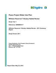
productivity, as well as inter-trophic interactions (Figure 1). The impact hypotheses, 

expressed here as null hypotheses (i.e., hypotheses of no difference or correlation), are 

tested separately for each reservoir and relate primarily to levels of primary productivity. 

H01: Average reservoir concentration of Total Phosphorus (TP), an indicator of 

general phosphorus availability, does not limit pelagic primary productivity. 

H02: Relative to the availability of phosphorus as measured by the level of total 

dissolved phosphorus (PO4), the average reservoir concentration of nitrate (NO3) 

does not limit pelagic primary productivity. Nitrate is the dominant form of 

nitrogen that is directly bio-available to algae and is indicative of the general 

availability of nitrogen to pelagic organisms. 

H03: Water retention time (τw) is not altered by reservoir operations such that it 

significantly affects the level of TP as described by Vollenweider’s (1975) 

phosphorus loading equations (referred to here as TP(τw)). 

H04: Water temperature, and hence the thermal profile of the reservoir, is not 

significantly altered by reservoir operations. 

H05: Changes in TP as a result of inter annual differences in reservoir hydrology (i.e., 

TP(τw)) are not sufficient to create a detectable change in pelagic algae biomass 

as measured by levels of chlorophyll a (Chla). [This hypothesis can only be 

tested if H03 is rejected] 

H06: Independent estimates of algae biomass based on TP(τw) and Secchi disk 

transparency (SD) prediction equations are statistically similar, suggesting that 

neither non-algal turbidity, nor intensive zooplankton grazing, are significant 

factors that influence standing crop of pelagic phytoplankton (Carlson 1980, cited 

in Wetzel 2001) 




H07: The effect of non-algal turbidity on pelagic algae biomass, as indicated by the 

difference in independent predictions of Chla by TP(τw) and SD (Carlson 1980, 

cited in Wetzel 2001), does not change as a function of reservoir operation. 

H08: The ratio of ultra-phytoplankton (< 20 µm in size) to micro-phytoplankton (20-200 

µm in size) abundance is not altered by reservoir operations and hence, does not 

change through time with the implementation of the WUP Combo 6 operating 

strategy. 

H09: The size distribution of the pelagic zooplankton population (an indicator of fish 

food bioavailability as larger organisms tend to be preferred over small ones) is 

not altered by reservoir operations and hence, does not change through time with 

the implementation of the WUP Combo 6 operating strategy. 

H010: Primary production, as measured through C14 inoculation, is not altered by 

reservoir operations and hence, does not change through time with the 

implementation of the WUP Combo 6 operating strategy. 

Hypotheses H01 to H07 examine and put into context the most likely pathways by 

which reservoir operations may impact primary productivity. Collectively, these 

hypotheses define a crude model of reservoir operation effects on pelagic primary 

productivity that will lead to a greater understanding of such impacts, and ultimately to a 

prediction of possible outcomes when future operational strategies are explored. A 

schematic of the model is shown in Figure 1. 

Reservoir 

Operations 

Nutrient 

Inflow 

Water 

Retention 

Temperature 

Profile 

Turbidity 

Nutrient Bioavailability 

Primary 

Productivity 

Secondary 

production 

Fish 

Productivity 

Figure 1: Schematic diagram of the pelagic impact hypothesis model illustrating 

how H01 to H08 inter-relate to affect primary productivity and ultimately 

fish productivity. Littoral productivity also plays a significant role, but 

is excluded from this illustration as it is dealt with in a separate 

monitor. 




Hypothesis H08 establishes the primary pathway by which carbon and other 

nutrients enter the food web, and reflects the general growing conditions of 

phytoplankton. A predominance of ultra-phytoplankton tends to indicate poorer growing 

conditions, which collectively include the influences nutrient levels, water temperature, 

light availability etc. (Wetzel 2001). Conversely, a predominance of micro-phytoplankton 

indicates an excellent growing environment. 

Hypothesis H09 explores the linkage between primary production and fish 

production by examining the size structure of zooplankton (secondary production). Of 

importance is the density of larger organisms that tend to constitute the majority of 

pelagic fish food production. 

Hypothesis H010 is an independent test of the impact hypothesis model as it 

pertains to the WUP Combo 6 operating strategy. 

1.4 Key Water Use Decision Affected 

In the absence of reliable predictions on the effect of dam operations on Stave 

reservoir productivity, it was assumed that pelagic productivity would remain unchanged 

over the spectrum of feasible reservoir operating strategies. However, the CC 

recognised that there was considerable uncertainty in this assumption, but had no 

information with which to form other, more probable outcomes. This monitor is designed 

to: 

a) Test the validity of this assumption of no operational impact, and confirm that 

pelagic conditions have not worsened with the new Combo 6 operating strategy. 

b) Provide the information necessary to promote a better understanding of the 

pathways by which operational changes can affect primary productivity (the 

chosen indicator variable of fish productivity), and in turn provide better 

predictions of operational impacts for future WUP reviews. 

In addition, this monitor attempts to develop a better linkage between the effect 

of reservoir operations on primary productivity and the potential for fish production. 

Collectively, this information will lead to conclusions regarding the expected 

benefits of the Combo 6 operating strategy, and whether alternative strategies should be 

proposed if these benefits are not realised. Through a better understanding of reservoir 

ecosystem dynamics, its may be possible to find improvements to the Combo 6 

operating strategy that may increase operational flexibility without compromising 

reservoir ecosystem function. Specific actions that may lead to such improvements 

cannot be identified at this time because of the complexity of the Stave Lake project. 

The complex modelling exercises needed to identify such actions is beyond the scope of 

this monitor and should be reserved for future WUP processes. 




2.0 Monitoring Program Proposal 

2.1 Objective and Scope 

The objective of this monitor is to collect the data necessary to test the impact 

hypotheses outlined in Section 1.3 and hence, address the management questions 

presented in Section 1.2. The following aspects define the scope of the study: 

a) The study area will consist on Stave Lake and Hayward Lake Reservoirs. 

b) Data will be collected at three sites; two on Stave Lake reservoir because of 

potential spatial gradients in light, wind an nutrient exposure, and only one on 

Hayward Lake reservoir which is much smaller and less prone to spatial 

heterogeneity. 

c) The program is to be carried out in two phases, an initial 2-3 year high intensity 

sampling program, and a subsequent base level sampling program. 

d) The monitor is to continue for 10 years or until the next WUP review period. 

e) The monitor will focus primarily on variables associated with measures of pelagic 

primary productivity, a component of reservoir productivity that is assumed to be 

a suitable indicator of overall productivity. 

2.2 Approach 

The general approach to the pelagic monitor is to identify the primary pathways 

by which reservoir operations may affect overall productivity, as indicated by changes in 

primary productivity, through impact hypothesis testing. The necessary physical, 

chemical and biological data will be collected to test each of the 9 hypotheses listed in 

Section 1.3. Depending on the acceptance or rejection of each hypothesis, a conceptual 

model will be developed to predict the direction of change in productivity for a given 

change in operation. If the conceptual model is proved valid, an attempt will be made to 

develop a numerical model to predict the magnitude of change. The success of this 

modelling exercise will be depend on the variability of the data collected, the variability of 

year to year reservoir operations and the strength of correlation among parameters. 

Data collection and analysis will proceed as a two-phased program. The initial 

phase will last 2-3 years and will involve an intensive data collection program designed 

to test all impact hypotheses listed in Section 1.3. During this phase, light intensity, 

Secchi Disk depth, water temperature, oxygen level, daily solar irradiation, total 

dissolved phosphorus concentration, total nitrate concentration, chlorophyll a 

concentration, phytoplankton community structure, zooplankton community structure, 

and 14 C estimates of primary production will be collected at each study site every 6 to 8 

weeks. Because of the high cost of lab analysis, the set of 14 C estimates of primary 

production will only be done once every 3 years. At the conclusion of this phase, a 

report will be prepared that summarises the finding in terms of hypotheses H01 to H010, 

and attempts to construct conceptual and if possible, an initial numerical model of 

pelagic primary production in each reservoir. 




The next phase of the monitor will be of much lower sampling intensity, but will 

be carried out annually till the next WUP review process. During this phase, only light 

intensity daily solar irradiation, total dissolved phosphorus concentration, total nitrate 

concentration, chlorophyll a concentration and 14 C estimates of primary production will 

be collected. Sampling frequency will be reduced to 4 sampling periods per year (May 

to November), the dates of which are to be set according to annual patterns uncovered 

in Phase 1 of the monitor. These data are not only going to be useful in testing and 

refining models developed in Phase 1, but will be used to track pelagic productivity over 

time to determine whether there are changes in response to annual differences in 

reservoir operation. As well, these data will be incorporated into the littoral productivity 

monitor to track the ratio of littoral to pelagic production and how it may affect overall 

reservoir productivity (Wetzel 2001). 

It should be noted that the data collection component of Phase 1 has been 

completed, and an initial data report has been prepared (Stockner and Beer 2004). 

However, QAQC of the data and hypothesis testing have not been done, nor have the 

modelling exercises been started. 

2.3 Methods 

The scope of the monitor, the parameters to be measured and the frequency of 

sampling have already been discussed in the preceding sections. The sections that 

follow will describe the method of data collection for each of the variables listed in 

Section 2.2. Because data collection for Phase 1 of the program has been completed, 

focus of this section will be on Phase 2 of the monitor, and the methods will be described 

in sufficient detail to ensure consistency between phases. 

2.3.1 Water Quality – Physical Variables 

Light intensity (µmole quanta m -2 s -1 ), will be measured at 1 m intervals to a depth 

beyond the point at which photosythetically active radiation PAR (light with a wavelength 

between 400 to 700 µm) is 1% that of the surface or to the lake bottom, whichever is 

reached first. It is essential that the sensor be vertical, and that the boat does not cast a 

shadow over the sensor while being lowered. A 0 m reading (a film of water should be 

on the surface of the sensor) should be taken prior to and immediately following the 

sensor reading at depth. The LiCor Model Li-250 submersible quantum sensor is highly 

recommended for this application to maintain consistency with historical measurements. 

Vertical profiles of PAR will be natural-log transformed and plotted against depth to 

obtain an estimate of the light extinction coefficient (k). Vertical profiles will be collected 

every 8 weeks to define the annual cycle of the euphotic zone – the volume of water that 

is capable of sustaining photosynthetic activity, as well as the cycles for light 

compensation depth and the light extinction coefficient. The latter two variables, in 

conjunction with Secchi disk readings taken with a 20 cm weighted disk on the shaded 

side of the boat, will be incorporated into the pelagic productivity diagnostic tool 

developed by Carlson (1980) (cited in Wetzel 2001) to test hypothesis H06. The latter 

two variables will also be used in the littoral monitor. 




Water temperature (°C) and oxygen level (O2, mgL -1 ) will be measure at 1 m 

intervals to a depth just beyond the thermocline, and then at 5 m intervals to the lake 

bottom (i.e., sediment surface). It is essential that the O2/temp sensor be calibrated and 

kept vertical by use of a lead weight for each sampling occasion. The temperature data 

will be used to define the epilimnetic zone, a parameter necessary to model nutrient 

dynamics during period of thermal stratification. The O2 data will be used to monitor O2 

deficits in the hypolimnion and provide an indication of potential nutrient availability at 

times of lake-turnover. In Phase 1, vertical profiles of water temperature and O2 will be 

carried out every 4 to 6 weeks to capture annual cycles in stratification. Sampling 

frequency will then drop to every 8 weeks during the months of May to November for 

Phase 2 of the monitor. 

In addition to the in situ variables above, data on total daily solar irradiation will 

be collected from the Greater Vancouver Regional District who operates a LI-200SA 

pyranometer in Port Moody. This data will be used to monitor daily fluctuations in total 

solar irradiation, and hence correct for daily/annual fluctuations in potential 

photosynthetic productivity when comparing samples. 

2.3.2 Water Quality – Chemical 

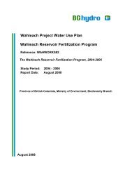
Water quality samples at each of the sample sites (Figure 2) will be collected by 

a vertical, non-metallic Van Dorn sampler at 1, 3 and 5 m depths below the water 

surface. The three ~ 500 ml samples will be poured in a large (2 L) dark bottle and then 

mixed to get a single representative sample for the site. All samples/site for water 

quality analysis will be drawn from this mixed epilimnetic sample. 




To analyse total phosphorous (TP) content, the TP sample test tubes and caps 

(one per site) will first be rinsed with the sampled water, and then filled, capped and 

labelled. At no time will the mouth of the bottle or the inside of the cap be touched, as it 

can easily become contaminated. Once filled, the sample test tubes should be placed in 

a cooler and then refrigerated until analysed. Once per field trip, two sample bottles of 

double distilled water (DDW) will be prepared as blanks for comparison purposes. 

Figure 2: Map of Stave Lake and Hayward Lake reservoirs showing monitor sampling 

locations 




In preparation for dissolved phosphorus and nitrogen (in the form of N03) 

analysis, the mixed epilimnetic water sample will be field filtered using a 47 mm filtering 

manifold equipped with an ashed GF/F filter. Prior to filtering, the filter will be rinsed with 

180 ml of DDW, and then rinsed again with 180 ml of the sampled epilimnetic water. 

Plastic 120 ml sample bottles will be rinsed by filtering 60 ml of the Van Dorn sampled 

water into each bottle, which will then be capped and shaken. All filtrate to this point will 

be discarded. The rinsed sample bottles will then be filled with filtered epilimnetic water, 

capped tightly, and immediately frozen. Once per field trip, two sample bottles of double 

distilled water (DDW) will be prepared as blanks for comparison purposes. 

During Phase 1, water quality samples will be collected every 4-6 weeks to 

determine annual trends. In phase 2, sampling frequency will be reduced to 4 times per 

year (every 8 weeks during months of May to November). All samples will be to be sent 

immediately to a certified chemistry laboratory for analysis. For consistency purposes it 

is recommended that the Department of Fisheries and Oceans chemistry lab in Cultus 

Lake should be used. The data obtained from this analysis will be used to test 

hypotheses H01, H02, and H05 to H07 in Section 1.3. 

2.3.3 Plankton 

Phytoplankton 

Phytoplankton community structure will be determined by visual assessment of 

water samples collected by vertical Van Dorn sampler at depths 1, 3, and 5 m below the 

water surface. Each sample will be stored in 250 ml glass bottles to which 2 ml of acidic 

Lugol’s iodine solution has been added as a preservative. Samples are to be stored in a 

cool dark location until analysed. Sampling at each site (Figure 2) will occur monthly 

between March and November each year. Only one sample per site will be taken and 

analysed. 

Prior to enumeration by the Utermohl (1958) method, the sample will be shaken 

for 60 s, poured into 25 ml settling chambers, and then allowed to settle for a minimum 

of 8 hr. Counts should be done with an inverted phase-contrast plankton microscope. 

Counting will follow a two step process starting with an enumeration of microphytoplankton 

(e.g., diatoms, dinoflagellates, and blue-green algae) in the first 5-10 

random fields at a microscope magnification of 250X. This will be followed by a random 

transect (10-15 mm in length) count where magnification is increased to 1560X to 

enumerate ultra-phytoplankton (e.g., pico-cyanobacteria and nano-flagellates). In total, 

a minimum of 250 cells will be counted per sample to ensure statistical accuracy. All 

enumerated cells will be identified to the nearest species taxon level. Counts will be 

reported as an abundance value (cells·ml -1 ) and in terms of biovolume (mm 3 L -1 ). 

During phase 1 of the monitor, phytoplankton enumeration will be carried out 

every 4 to 6 weeks each year to capture seasonal and annual trends. The level of 

phytoplankton sampling effort will be reduced to just one sample per site, per year for 

Phase 2 of the monitor. The maximise the utility of the phase 2 samples, it will have to 




be collected at the same time of year, preferable during late summer when the when 

reservoir levels are consistent between years due to recreational constraints. The data 

will be used to test hypothesis H08 of the monitor. 

Chlorophyll 

In addition to the phytoplankton counts, water samples will be collected to 

estimate chlorophyll a concentration, an indicator of phytoplankton standing crop. At 

each station, 500 ml water samples will be collected at 1, 3, and 5 m below surface, and 

mixed together in a large dark glass bottle to yield a single depth integrated sample. 

Starting with 500 ml of the mixed epilimnetic water, field-filter the sub-sample using a 

47 mm filtering manifold with a 0.45 µm Millipore HA filter. Should the filter become 

plugged, discard the sub-sample and re-start the filtering process with a new 250 ml 

sub-sample. At no time should the vacuum pressure of the filtering mechanism exceed 

20 cm Hg. When dry, the filter should be folded, placed in small round aluminium 

dishes, and kept frozen until analysed. 

During phase 1 of the monitor, Chlorophyll samples will be collected every 4 to 6 

weeks to capture annual trends in phytoplankton standing crop. In Phase 2, the level of 

sampling effort will be reduced to 4 times per year (every 8 weeks between May and 

November). All samples will be to be sent immediately to the Department of Fisheries 

and Oceans chemistry lab in Cultus Lake for analysis. The data obtained from this 

analysis will be used to test hypotheses H05 and H07 in Section 1.3. 

Zooplankton 

Zooplankton samples will be collected by Wisconsin vertical trawl hauls at each 

sample station (Figure 2). The Wisconsin trawl net, which should not have a mesh size 

greater than 80 µm and a throat diameter of 50 cm, will be lowered to a depth of 30 m 

and hauled up at a speed of 0.5 m·s -1 . Once out of the water, the net should be rinsed 

with a wash bottle to ensure that all organisms are in the collecting cup (cod-end). The 

contents of the collecting cup are then washed into a plastic storage bottle to which 

ethanol has been added as a preservative. 

Prior to enumeration, the total volume of the sample will be stirred and split with a 

Folsom splitter to a volume that contains at least 100 post nauplii stages of the most 

abundant taxa. Enumeration will be done on a gridded petri-dish using a stereo 

microscope under suitable magnification. Taxonomic identification will be taken to the 

species level. Body length of individuals will be measured to the nearest 0.1mm, and 

then using published length weight relationships (McCauley 1984) assign an 

approximate dry weight (µg). The resulting data will then be used to determine species 

density (No·L -1 ) and biomass (µg·L -1 ), as well as overall length distributions. These data 

will then be used to test hypothesis H09. 

During phase 1 of the monitor, zooplankton enumeration will be carried out every 

4 to 6 weeks each year to capture seasonal and annual trends. In phase 2 of the 

monitor, zooplankton sampling effort will be reduced to just one sample per year, and 




analysis will be limited to the development of a length frequency distribution (no 

identification will occur beyond the family level of taxon). The maximise the utility of the 

phase 2 samples, it will have to be collected at the same time of year, preferable during 

late summer when the when reservoir levels are consistent between years due to 

recreational constraints. The data will be used to test hypothesis H08 of the monitor. 

2.3.4 14 C Estimate of Primary Production 

Primary production (mgC·m -2 d -1 ) will be estimated by H 14 CO3 inoculation as 

described by Strickland (1960). Water samples will be collected by Van Dorn sampler at 

1, 3, 5, 7, and 10 m depths. Each depth-sample will be transferred equally to three 

300 ml BOD (Biological Oxygen Demand) bottles, the first two of which are clear to allow 

photosynthetic uptake of C 14 . The third bottle is darkened to exclude light so as to 

measure C 14 uptake through respiration alone. Each of the sample bottles will be 

inoculated with 1 ml of 3.7 µCIE·ml -1 · 14 C-HC03 using a 1 ml Eppendorf pipette with 

disposable tips (the fist aliquot of C 14 from a freshly filled tip should be discarded). After 

inoculation, the sample bottles will be to be lowered to their respective collection depths 

and incubated for 2-3 hr. Incubation should be initiated as close to 10 am as possible, 

but not allowed to continue beyond 1 pm. Following incubation, the inoculated samples 

are to be retrieved and placed into a light-tight metal box for storage. 

Within 4 hours of collection, the inoculated samples should be filtered through a 

0.2 µm, 47 mm diameter, polycarbonate membrane filter. Once filtered, the filters are 

transferred to scintillation vials where 4 drops of 6N HCL are added. After addition of the 

scintillation fluor, the vials are to be sent to the Radiation Laboratory at the University of 

British Columbia where analysis of beta activity (an indicator of 14 C update) will be 

carried out on a Beckman© Beta scintillation counter using standard protocols. Raw 

primary production estimates will be reported as depth specific mg 14 C·m -2 hr -1 , but be 

integrated across all water depths when discussing daily production rates (i.e., mgC·m - 

2 d -1 ). The daily primary production values will be used to test hypothesis HO10 in Section 

1.3 and will only be collected 4 times per year every three years (starting in year three of 

the monitor). 

2.3.5 Safety Concerns 

A safety plan will have to be developed for all aspects of the study in accordance 

to BCH procedures and guidelines. Of particular concern are the safety protocols 

surrounding the transport and use of low level radioactive materials such as 14 C. Only 

licensed practitioners can purchase the radioactive 14 C product needed for the 

inoculation procedure. As well, investigators that perform the inoculations must also be 

appropriately certified to handle and transport the material. 




2.3.6 Data Analysis 

Phase 1 

All data will be entered into Excel spreadsheets for analysis and presentation. 

Physical and chemical attribute data from the pelagic sample sites of each reservoir will 

be summarised using descriptive statistics and analysed for annual trends. The data will 

also be used to test hypotheses H01 to H07 based on published criterion and trophic 

level relationships. Between-site and between-reservoir comparisons will only be 

descriptive in nature, as there are no replicates to estimate sample variance for 

statistical testing. 

Plankton identification and enumeration data will be similarly summarised in 

tables for between-site and between-reservoir comparisons. Also of interest would be 

tests for annual trends in community structure, as well as analyses of depth distributions 

of key classes of phytoplankton. The data will also be used to test hypotheses H08 and 

H09. 

The 14 C estimates of pelagic primary production will be the first in a series to be 

collected over the next 10 years. Because only a single data set will exist, primary 

production will only be discussed relative to between-site and between-reservoir 

differences, as well as indications of an annual trend. Test of H010 will have to wait for 

until sufficient yearly samples are collected. 

The modelling exercise will utilise multiple linear regression techniques to relate 

various summary descriptors of reservoir hydraulics to summary statistics of nutrient 

concentration, chlorophyll level, and when possible primary production. Where 

necessary, assumptions of linearity, normality, homoscedasticity, independence and 

randomness will be assessed prior to proceeding with analyses to ensure that statistical 

tests are being used appropriately. This test of assumptions applies to all statistical 

testing used in the monitor. 

Phase 2 

Data analysis in Phase 2 will consist of two parts. The first set of analyses will be 

to compare annual predictions of 14 C based primary production and other limnological 

variables made by the pelagic model with those collected in the field. The comparison 

will provide an indication of the model’s validity and utility as well as provide a means to 

annually refine the model’s predictive power with new data. The analysis and modelling 

exercise will employ the same analytical tools as used in Phase 1 of the monitor. 

The other component of the analysis will be to track pelagic primary productivity 

over time in each reservoir, and hence test hypothesis H010. The test will be carried out 

every three years of the monitor. With each compilation of 14 C primary production 

estimates, an attempt will be made to develop a predictive model so as to interpolate 

primary production between sampling periods. Like Phase 1, the modelling will rely on 

multiple linear regression techniques to test for possible relationships. 




As in Phase 1, assumptions of linearity, normality, homoscedasticity, 

independence and randomness will be assessed prior to proceeding with analyses to 

ensure that all statistical tests are being used and interpreted appropriately. 

2.3.7 Reporting 

At the end of each year during the first phase of the monitor, a data summary will 

be prepared that document the year’s findings. At the conclusion of Phase 1, two 

reports will be prepared, the first of which summarises the data collected to date. The 

second report will present and discuss the results of the hypothesis testing exercise, as 

well as present conceptual and if possible numerical models of reservoir primary 

productivity. Both reports will be submitted to the Management Committee for review 

prior to being finalised for general release. 

As in Phase 1 of the monitor, annual data reports will be prepared to summarise 

annual findings, each including a discussion of the year’s data relative to those collected 

in previous years. Part of this discussion will be an assessment of increasing or 

decreasing temporal trend. Prior to finalising the annual reports, the Management 

Committee will be given an opportunity to review then and provide comments. 

At the conclusion of the monitor, a comprehensive report will be prepared from 

the Phase 1 reports and all of the annual data reports that: 

a) Re-iterates the objective and scope of the monitor, 

b) Presents the methods of data collection, 

c) Describes the compiled data set and presents the results of all analyses, and 

d) Discusses the consequences of these results as they pertain to the current WUP 

operation, and the necessity and/or possibility for future change. 

Like the annual data reports, the Management Committee will review a draft of the final 

report prior to its general release. 

2.4 Interpretation of Monitoring Program Results 

Monitoring program results will be interpreted in two different ways. The first of 

these will be in terms of identifying the pathway(s) by which reservoir operations affect 

primary production in both Stave and Hayward reservoirs - the focus of Phase I of the 

monitor. It is anticipated that the differences in operation between reservoirs, as well as 

inter annual variability in operations will provide sufficient contrast to detect trends if 

such exist. If trends are inconclusive, then it will be considered safe to assume that 

reservoir operations within the range that was experienced during Phase 1 of the 

monitor do not affect primary production. Conversely, if measurable trends are found, 

analytical techniques will be employed to develop both conceptual and if possible, 

numerical models, that will useful in future WUPs for predicting the outcome of 

alternative operating strategies 




The monitor will also be interpreted in terms of accepting or rejecting the 

assumption made during the WUP process that pelagic productivity does not change in 

response to reservoir operations. This assumption was adopted largely because of a 

lack of information that indicates otherwise. Though CC members were tempted to 

assume some sort of causal relationship, there was too little data available to determine 

its general nature with any degree of certainty. A direct test of this assumption through 

annual comparisons of primary production estimates, in conjunction with the result of 

Phase 1 of the monitor, will lead to its rejection or validation. 

If deemed valid, the impetus will be to explore the possibility of relaxing reservoir 

constraints as an option in future WUPs. However, if deemed invalid, the models and 

monitor information can be used to assess the benefits of further constraining reservoir 

operations and enhance overall productivity. These constraints however, will be at the 

cost of other values in the system. To help resolve such conflicts, the results of the 

monitor may be used to develop appropriate non-operational alternatives. It should be 

stressed that the discussion of future actions will occur at the next WUP process. 

2.5 Schedule 

As indicated in section 2.2, much of Phase 1 has already been completed, but 

the final QA/QC of the data, as well as the hypothesis testing and modelling components 

of the monitor, have yet to be started. Part of the work in year 1 will be to finish the 

tasks of Phase 1, including a final report summarising all of the information and analyses 

as they pertain to the WUP. 

Because Phase 1 is near completion, Phase 2 of the monitor will also be started 

in year 1 of the monitor. Every three years, a 14 C estimate of primary production will be 

carried out until the end of the monitor at the next WUP review process - a period of 10 

years. 

2.6 Budget 

The total cost of the monitor is estimated to be $269,900. Roughly $10,200 of 

this amount is to cover the costs of completing Phase 1 of the monitor while the 

remainder is for carrying out Phase 2. The annual cost will cycle between $22,500 and 

$33,900 per year depending on whether a 14 C estimate of primary production is done. 

Average annual cost of the 10-year monitor is $26,000 per year, a value within $1000 

(4%) of the proposed cost listed in the CC report (Failing1998). 

The costs given above are based on the cost of services and products in 2004. 

When adjusted for annual inflation (2%), the total program cost is expected to be closer 

to $300,800. A summary breakdown of the labour costs and expenses is provided in 

Table 1-1. 




Table 1-1: Estimated costs for the pelagic productivity monitor. Contingency is calculated on field labour, and covers safety planning, 

regulatory approvals (permits), field logistics, and unforeseen weather delays 

Task Labour 

Daily 

Rate 

Units per year 

Yr 1 Yr 2 Yr 3 Yr 4 Yr 5 Yr 6 Yr 7 Yr 8 Yr 9 Yr 10 

Project Management Project Manager $ 700 1 1 1 1 1 1 1 1 1 1 $ 7,000 

Field Data Collection Sr. Biologist $ 850 2 1 2 1 1 2 1 1 2 1 $ 11,900 

Project Biologist $ 600 4 4 4 4 4 4 4 4 4 4 $ 24,000 

Technicien 2 $ 300 4 4 4 4 4 4 4 4 4 4 $ 12,000 

Data Entry Technicien 1 $ 300 2 2 2 2 2 2 2 2 2 2 $ 6,000 

Data Analysis Sr. Biologist $ 850 2 1 1 1 1 1 1 1 1 1 $ 9,350 


Reporting Sr. Biologist $ 850 2 1 2 1 1 2 1 1 2 1 $ 11,900 


Technicien 1 $ 500 14 8 8 8 8 8 8 8 8 8 $ 43,000 

Contingency 5% $ 1,390 $ 903 $ 1,018 $ 933 $ 903 $ 1,018 $ 903 $ 903 $ 1,018 $ 903 $ 9,888 

Total Labour $ 29,190 $ 18,953 $ 21,368 $ 19,583 $ 18,953 $ 21,368 $ 18,953 $ 18,953 $ 21,368 $ 18,953 $ 207,638 

Expenses 

Unit 

Cost 

Vehicle (per km) $ 0.45 1000 1000 1000 1000 1000 1000 1000 1000 1000 1000 $ 4,500 

Boat Rental $ 250 4 4 4 4 4 4 4 4 4 4 $ 10,000 

Chlorophyll a $ 25 12 12 12 12 12 12 12 12 12 12 $ 3,000 

Nutrients $ 65 12 12 12 12 12 12 12 12 12 12 $ 7,800 

Phytoplankton $ 165 3 3 3 3 3 3 3 3 3 3 $ 4,950 

Zooplankton $ 50 3 3 3 3 3 3 3 3 3 3 $ 1,500 

14 

C (per sample) $ 150 

60 60 60 $ 27,000 

sample vials $ 5 30 30 30 30 30 30 30 30 30 30 $ 1,500 

Report reproduction $ 200 1 1 1 1 1 1 1 1 1 1 $ 2,000 

Total Expenses $ 3,525 $ 3,525 $ 12,525 $ 3,525 $ 3,525 $ 12,525 $ 3,525 $ 3,525 $ 12,525 $ 3,525 $ 62,250 

Program Total $ 32,715 $ 22,478 $ 33,893 $ 23,108 $ 22,478 $ 33,893 $ 22,478 $ 22,478 $ 33,893 $ 22,478 $ 269,888 

Inflation Adjustment 2% $ 33,368 $ 23,385 $ 35,966 $ 25,011 $ 24,816 $ 38,167 $ 25,819 $ 26,335 $ 40,504 $ 27,399 $ 300,770 

BC Hydro Page 21 

10-year 

Total



2.7 References 

Carlson, R. E. 1980. More implications in the chlorophyll-Secchi disk relationship. 

Limnol. Oceanogr. 25:378-382. (Cited in Wetzel 2001) 

Failing, L. 1999. Stave River Water Use Plan: Report of the consultative committee. 

Prepared by Compass Resource Management Ltd for BC Hydro. October 1999. 

44 p + App. 

McCauley, E. 1984. The estimation of the abundance and biomass of zooplankton in 

samples. In: Downing, J.D. and F. H. Rigler (eds). 1984. A Manual on Methods 

for the Assessment of Secondary Productivity in Fresh Waters – 2nd ed., 

Blackwell Scientific Publications. 

Strickland, J. D. H. 1960. Measuring the Production of marine phytoplankton. Bull. J. 

Fish. Res. Baord Can. 122, 172 p. 

Stockner, J. G. and J. Beer. 2004. The limnology of Stave/Hayward reservoirs: with a 

perspective on carbon production. Prepared for BC Hydro Water Use Plans by 

Eco-logic Ltd. and University of British Columbia, Institute For Resources, 

Environment and Sustainability, Vancouver. 33 p. + App. 

Utermohl, H. 1958. Zur Vervollkommnung der quantitativen Phytoplankton methodik. 

Int. Verein. Limnol. Mitteilungen No. 9. (Cited in Stockner and Beer 2004) 

Vollenweider, R, A. 1975. Input-outout models, with special refernce to the phosphorus 

loading concept in limnology. Schweiz. Z. Hydrol. 37:53-84. (Cited in Wetzel 

2001) 

Wetzel, R. G. 2001. Limnology: Lake and River Ecosystems 3 rd Edition. Academic 

Press. New York. 1006 p. 






2. Littoral Productivity Assessment 

During the Stave River Water Use Plan process, the consultative committee (CC) 

identified the need to study the effects of water level fluctuation on the littoral zone 

productivity of Hayward and Stave reservoirs. This requirement arose largely from 

concerns raised by fisheries interests that the littoral zone in Stave reservoir may have 

been seriously damaged by water level fluctuations. It was further hypothesised that the 

loss of a fully functional littoral zone could have significantly impacted the overall 

biological (carbon) production of the ecosystem. These concerns however, were not 

based on actual measures of impact. From site visits and comparisons to unaltered lake 

systems, it was clear that the water level fluctuations in Stave Reservoir have had a 

serious impact on littoral productivity. However, the full extent and nature of the impact 

remains to be quantified. Also uncertain was how this loss/gain relates to productivity 

levels of the system as a whole (i.e., to what extent does littoral productive contribute to 

overall system productivity?). 

In an attempt to account for this potential loss in system productivity for trade-off 

analysis purposes, a performance measure was developed that estimates the areal 

extent of ‘potentially productive’ littoral habitat. The measure, termed the ‘Effective 

Littoral Zone’ or ELZ, quantifies the area of aquatic shoreline habitat that receives 

adequate light to promote photosynthetic activity and remains wetted for specified 

occurrence frequencies. A description of how the measure is calculated can be found in 

Appendix 2 of the consultative committee report (Failing 1999). Although the ELZ 

performance measure was used during the development of the WUP, its accuracy as a 

measure of productive littoral habitat remains untested. 

The Stave River generation complex provides a unique opportunity to test the 

utility of ELZ measure. The complex consists of three reservoirs, two of which have 

highly variable water levels, while the other is kept relatively stable. The contrast in 

operation between reservoirs allows one to compare ELZ predictions with empirical data 

collected under differing degrees of reservoir stability. The loss of the littoral zone was 

deemed to be an extremely important issue by the CC. However, decisions made about 

reservoir operations in the WUP were based on an untested measure of this loss. As a 

result, a comprehensive study of littoral zone impacts, and the ELZ measure used to 

quantify it, was deemed an essential component of the WUP. The results of the study 

would be used in future Stave River WUPs to clarify the issues surrounding this loss of 

littoral zone productivity. It may also lead to the development of a littoral zone 

productivity performance measure that could be transferable to other BCH facility WUPs. 

At the conclusion of the WUP process, the CC reached a consensus to adopt the 

Combo 6 operating strategy as the preferred alternative for the next ten years (Failing 

1999). One of the reasons the alternative was chosen was because of the expected 




benefits in littoral habitat. Because relevance of the ELZ measure was untested, the CC 

expressed concern whether the perceived littoral benefit would actually be realised. As 

a result, the CC also recommended that a monitor be designed and implemented to 

measure changes in littoral zone development following implementation of the Combo 6 

operating strategy. 


The consultative committee identified four key management questions that must 

be addressed pertaining to the littoral productivity of Stave and Hayward reservoirs. 

These are: 

a) What is the current level of littoral productivity in each reservoir, and how does it 

vary seasonally and annually as a result of climatic, physical and biological 

processes, including the effect of reservoir fluctuation? 

This information is required to identify the key determinants that currently 

govern/constrain the littoral productivity in each reservoir. Once these 

environmental factors have been identified, an assessment can be carried out to 

determine whether they are susceptible to change given alternative reservoir 

management strategies. Environmental factors that are susceptible to change 

are then monitored through time in conjunction with the productivity indicator 

variable (in this case primary productivity). This information sets up the 

foundation for the next management question. 

b) If changes in littoral productivity are detected through time, can they be attributed 

to changes in reservoir operations as stipulated in the WUP, or are they the 

result of change to some other environmental factor? 

This information allows one to determine whether there is a significant, causal 

link between reservoir operations and reservoir littoral productivity, and if so, 

describe its nature for use in future WUP processes, particularly in the context of 

the ELZ performance measure. Implicit in this question is that gains or losses in 

primary productivity reflect gains or losses in overall fish production. 

c) A performance measure was created during the WUP process so as to predict 

potential changes in littoral productivity based on a simple conceptual model. 

The Effective Littoral Zone (ELZ) performance measure was used extensively in 

the WUP decision making process, but its validity is unknown. Is the ELZ 

performance measure accurate and precise, and if not, what other environmental 

factors should be included (if any) to improve its reliability? 

The ELZ performance measure is purely a conceptual construct at this stage. 

Because decisions were made based on the values of this performance 

measure, it is imperative that it be validated in terms of its accuracy, precision, 

and reliability. Because littoral productivity is affected by reservoir operations 

elsewhere in the province, the ELZ tool may prove useful in other WUPs. Its 

transferability to other reservoirs should also be investigated. 




d) To what extent would reservoir operations have to change to 1) illicit a littoral 

productivity response, and 2) improve/worsen the current littoral and overall 

productivity levels? 

e) Does the Combo 6 operating alternative improve reservoir littoral productivity as 

was expected in the WUP. Is there anything that can be done to improve the 

response, whether it be operations-based or not? 

This is a compliance component of the monitor and is designed to assess 

whether the expected increase in littoral productivity was realised. 


Measures of littoral productivity in lacustrine environments are difficult, and 

therefore costly to obtain directly. As a result, the CC recommended that a weight-ofevidence 

approach be used to examine the relationship between littoral productivity and 

reservoir operations. This approach relies on a series of impact hypothesis tests to 

construct a likely model that describes the causal relationship, should one exist. The 

impact hypotheses, expressed here as a set of null hypotheses (i.e., hypotheses of no 

difference or correlation), are tested separately for each reservoir and relate to levels of 

primary productivity as an indicator of potential fish productivity. The impact hypotheses 

are such that they can be grouped to deal with a common issue. 

The first set is almost identical to the first five hypotheses identified in the pelagic 

monitor, except that they rely on irradiance and chlorophyll data collected in the littoral 

zone rather than at pelagic sites. These hypotheses collectively try to identify the extent 

to which nutrient concentrations limit the potential maximum level of productivity in the 

littoral zone. These tests provide context to the overall analysis, but more importantly 

they are an attempt to take into account the confounding role of nutrient limitation on the 

outcome and interpretation of the monitor. The impact hypotheses are as follows: 

H01: Average reservoir concentration of Total Phosphorus (TP), an indicator of 

general availability of phosphorus is not limiting to littoral primary productivity. 

[Relies on data collected during the pelagic monitor and assumes that nutrient 

concentrations are uniform through out each reservoir] 

H02: Relative to the availability of phosphorus as indicated by level of total dissolved 

phosphorus (PO4), the average reservoir concentration of nitrate (NO3) is not 

limiting to littoral primary productivity. Nitrate is the dominant form of nitrogen 

that is directly bio-available to algae and higher plants and is indicative of the 

general availability of nitrogen to littoral organisms. [Relies on data collected 

during the pelagic monitor and assumes that nutrient concentrations are uniform 

through out each reservoir] 

H03: Water retention time (τw) is not altered by reservoir operations such that it 

significantly affects the level of TP as described by Vollenweider’s (1975) 

phosphorus loading equations (referred to here as TP(τw)). [Relies on data 




collected during the pelagic monitor and assumes that nutrient concentrations 

are uniform through out each reservoir] 

H04: Water temperature, and hence the thermal profile of the reservoir, is not 

significantly altered by reservoir operations. [Relies on data collected during the 

pelagic monitor and assumes that nutrient concentrations are uniform through 

out each reservoir] 

H05: Changes in TP as a result of reservoir operations (through changes in τw) are not 

sufficient to create a detectable change in littoral algae biomass as measured by 

littoral levels of chlorophyll a (CHL). [Relies on data collected during the pelagic 

monitor and assumes that nutrient concentrations are uniform through out each 

reservoir] 

The next suite of hypotheses deals with the general premise that littoral 

productivity in clear, low nutrient lakes tends to be much greater than pelagic 

productivity, and hence defines the productivity of the system as a whole. Underlying 

this premise is the theory that in clear, low nutrient systems, incoming nutrients are 

quickly assimilated into the littoral zone before getting a chance to work their way to the 

pelagic zone via the littoral food web. Conversely, when turbid conditions exist, the low 

light levels inhibit littoral growth and thus allow pelagic productivity to prevail. Similarly, 

when eutrophic conditions exist, the ability for the littoral system to sequester nutrients is 

overwhelmed, also allowing the pelagic system to flourish. As pelagic productivity 

increases, the high biomass reduces light penetration and in turn begins to inhibit 

productivity in the littoral zone. This feedback mechanism allows the pelagic zone to 

eventually dominate overall lake productivity (Wetzel 1983, Dodds 2003, Liboriussen 

and Jeppensen, 2003). 

Included in this suite of hypotheses is a test of the premise that nutrient cycling 

processes in the littoral zone slows the overall loss of phosphorus (either by outflow or to 

hypolimnetic sediments), and therefore, increases overall lake productivity compared to 

similar systems without a substantial littoral zone (Wetzel 1983). 

During the WUP, it was assumed that the two theories above applied to the 

Stave-Hayward system, and that the importance of the littoral zone to overall system 

productivity was deemed to be very high. The Stave–Hayward reservoir system 

however, is not a shallow water lake system. Also, the two reservoir systems tend to be 

very steep sided, so that the aerial extent of the littoral habitat may not be very large, 

even under ideal hydraulic conditions. Because of these two reasons, it is possible that 

the assumed theoretical importance of littoral zone productivity may be incorrect for 

these two reservoirs. 

Fortunately, the Stave-Hayward reservoir system does provide a unique 

opportunity to test this assumption. The Stave Lake reservoir, under present conditions, 

has limited littoral development because of the extensive drawdown events that it 




experiences. Hayward reservoir on the other hand, tends to be quite stable. If the 

assumption is indeed correct, then the following two hypotheses would hold true: 

H06: Overall primary production (as measured by 14 C inoculation and/or as inferred 

from ash free dry weight data) of Stave reservoir is less than that of Hayward 

Lake 

H07: Pelagic primary production dominates in Stave reservoir while littoral production 

dominates in Hayward reservoir. 

With the new WUP regime, the frequency and extent of drawdown in the Stave 

system is expected to decrease, while that of the Hayward system is likely to increase. 

Based on the assumptions that lead to the development of the ELZ performance 

measure (Appendix 2 of Failing 1999), these changes are expected to alter the quantity 

of littoral habitat suitable for primary production, and hence have an impact on overall 

system primary production. The extent with which this may occur, if indeed a response 

occurs at all, is uncertain. The test of this premise is the subject of the final set of 

hypotheses. It is important to note that in testing these hypotheses, one is also testing 

the validity of the ELZ measure. The null hypotheses are: 

H08: Stable reservoir levels do not lead to maximum littoral development as measured 

by 14 C inoculation and/or inferred from ash free dry weight data. 

H09: Water level fluctuations that raise the euphotic zone (defined here as the depth at 

which photosythetically active radiation (PAR) is 1% that of the water surface) 

from lower elevations does not lead to a collapse of littoral primary production (as 

measured by 14 C inoculation and/or inferred from ash free dry weight data) that 

occurred near the prior 1% PAR depth. 

H010: Littoral zone productivity, as measured by 14 C inoculation and/or inferred from 

ash free dry weight data, remains unchanged as reservoir water level stability 

increases. 

H011: Changes in littoral productivity (as measured by 14 C inoculation and/or inferred 

from ash free dry weight data) are expressed primarily in terms of changes in 

areal extent as defined by upper and lower boundary elevations. Within these 

boundaries, primary production does not vary in proportion to accumulated PAR 

exposure under wetted conditions [this is the premise that has lead to the 

development of the ELZ performance measure]. 

1.4 Key Water Use Decisions Affected 

During the WUP process, the perceived loss of littoral habitat in Stave Lake 

reservoir was deemed to be critical with respect to the overall productive capability of the 

system. Among the options explored was a reservoir management strategy that 

imposed restrictions on the extent of drawdown in the reservoir so as to partially recover 

some of the lost littoral habitat. The modelling exercise however, showed that reservoir 

stabilisation options would come at a cost to downstream fish habitat values. As a 




result, the option was not explored further because the downstream habitat costs were 

deemed too high for what was judged to be an uncertain gain in reservoir productivity. 

Furthermore, the final reservoir management strategy accepted by the CC had within it 

constraints in downstream releases that inherently created a slightly more stable state in 

Stave reservoir. The CC agreed to study the consequences of the present WUP, and 

hence learn more about the littoral productivity response to water level stability, before 

exploring further the concept of imposing reservoir constraints in future WUP processes. 

Constraints to reservoir operations, should they be deemed necessary, will come 

at a high cost to many other values, including power, downstream habitat, and First 

Nations heritage issues. Clearly defining the relative importance of the littoral zone to 

over all reservoir productivity, as well as identifying the extent of recovery need to 

restore full productivity, will help to identify alternative solutions, whether they be 

operational or physical in nature, that are more cost effective. 






a) The study area will consist on Stave Lake and Hayward Lake Reservoirs. 

b) Data will be collected at four sites; three on Stave Lake reservoir because of 

potential spatial differences, and one on Hayward Lake reservoir. 

c) The program is to be carried out in two phases, an initial 2-3 year high intensity 

sampling program, and a subsequent base level sampling program. 

d) The monitor is to continue to the next WUP review period. 

e) The monitor will focus of variables associated with measures of littoral primary 

productivity, a parameter assumed to be a component of overall reservoir 

productivity. 

2.2 Approach 

The basic study design is to compare periphyton growth at various reservoir 

elevations in Stave Reservoir (a highly variable system) with the pattern found in 

Hayward Reservoir (a relatively stable system). Growth will be measured by repeatedly 

sampling periphyton biomass on artificial substrate. The artificial substrata will be 

mounted on cinder blocks that are placed along permanently established transect lines 

(Figure 2, Monitor 1) where they will be spaced roughly every 2 m in depth beginning at 

the ‘full pool’ elevation to a depth equivalent to the light compensation depth at minimum 

operating elevation. Periphyton growth will be characterised by several parameters, 

including chlorophyll concentrations, ash-free dry weight estimates of biomass accrual, 

14 C primary production, and species composition. 




Samples will be collected along three transects in Stave Reservoir, and only one 

transect in Hayward Reservoir. Stave Reservoir is a large system with high glacial (i.e. 

turbid) inflows at its upstream end. As a result, the potential exists that there may be 

longitudinal differences in light attenuation rates that in turn could affect the depthrelated, 

functional response of periphyton growth. Hayward Lake, on the other hand, is 

much smaller, is free of such glacial influences, and would likely experience less 

variability. 

Each transect will be considered as a single sampling unit. As a result, the 

comparisons between transects will only be descriptive in nature. Statistical analyses 

will be limited given that replicate samples will not be collected to calculate sample 

variance. 

As in the pelagic monitor, the littoral zone monitor will be carried out as a twophased 

program. The first phase will involve intensive data collection geared towards 

addressing hypotheses H01 to H011, but with particular focus on H08 to H011. Littoral 

sampling during this phase will done every 5 weeks from April to November and will 

involve all variables listed above. The 5-week interval is critical in this monitor, as it is 

the maximum time that artificial strata can be left in oligotrophic systems without losing 

periphyton growth to grazing or sloughing. As a result, the periphyton accrual data 

become accurate indicators of production and when calibrated to 14 C estimates of 

production, it can be used as a direct measure of production. One of the key outcomes 

of Phase 1 of the monitor will be a numerical model of seasonal littoral productivity 

potential based on the founding concepts of the ELZ performance measure. The 

likelihood of such an outcome will depend on the extent of between-reservoir 

differences, inter-annual variability in reservoir operations and littoral development. Also 

a key determinant of the outcome will be the strength of association between operations 

and the parameters chosen to define littoral development. 

The second phase of the littoral monitor will be far less data intensive and will 

focus primarily on annual tests of hypotheses H06, H07 and H010, though anecdotal 

observations concerning the other hypothesis will be documented. Phase 2 of the 

monitor will rely on the ELZ modelling done in Phase 1 to predict littoral area given the 

previous 5 weeks of operation for each reservoir, including a prediction of littoral 

productivity. These predictions will in turn be related to measured values of littoral 

primary production (from the accrual data) as a test of the littoral zone model (a test of 

H010). Results of these annual tests of the ELZ model will be used to refine the model if 

necessary and test hypotheses H06 and H07. This annual tracking of hypotheses H06 

and H07 will provide important insight into the importance of littoral habitat in coastal 

reservoirs, as well as it’s general relationship to reservoir operations. 

During Phase 2, all four transects will be sampled every 5 weeks as in Phase 1. 

At each transect, periphyton samples will be collected at all sample stations, but only 4 

samples will be retained for accrual analysis. The spacing of these samples along the 

transect will be such that it captures the spatial trend of maximum productivity as 




indicated by the ELZ model and in situ estimates of periphyton accrual. The 4 accrual 

samples will be used to estimate littoral productivity using the 14 C-calibration curve 

developed in Phase 1. Every three years, a subset of transects will be subject to 14 C 

inoculation to re-evaluate, and correct if necessary, the accrual – primary productivity 

calibration curve. 

It should be noted that data collection for Phase 1 has already been done, and 

an initial data report has been prepared (Beer and Stockner 2004). However, QAQC of 

the data and hypothesis testing relative to WUP objectives have not been done, nor 

have the modelling exercises been started. In addition, none of the 14 C-inoculation work 

has been done. 

2.3 Methods 

2.3.1 Field methods 

Periphyton Growth Substrata 

Because of the difficulty in uniformly sampling a natural substrata (e.g. sediment 

surface, macrophytes, rocks, woody debris, etc.) with adequate replication, the method 

of choice to collect periphyton samples will be the use of artificial substrata (e.g. 

Plexiglas plates, glass slides, Styrofoam sheets, wooden sticks, etc.). In the present 

study, Plexiglas plates will be used. These plates will be attached to concrete blocks 

(25-30 kg) placed or dug into the sediment along a transect line that extends from the 

‘splash’ zone to 1m below the mean compensation depth (1% light level) of the reservoir 

at low pool (see Figure 2-1). The blocks will be placed at depth intervals between 1.5 

and 2 m. 

The Plexiglas plate will be elevated above the anchor block to permit movement 

of water on both sides. The surface of each plate will be scored with fine sandpaper to 

create a surface suitable for algae attachment. Plates will also be scored with a 

diamond pen into ‘quadrants’ to permit accurate quantitative sampling (see inset, Figure 

2-1). A 10 x 10 cm quadrant (100 cm 2 ) usually supplies sufficient periphyton to easily 

detect temporal changes in biomass and species composition in most oligotrophic lakes 

or reservoirs (Shortreed et al. 1984). To monitor accrual rates, quadrant sizes need not 

be as large. For the present study, the accrual quadrants were only 2.5 x 10 cm (25 

cm 2 ) in size. Thus, each plate was partitioned into three 100 cm 2 quadrants, each to 

sample for species composition, Chlorophyll a and ash free dry weight biomass 

estimates, and eight 25 cm 2 quadrants to carry out accrual sampling (see below). 

During Phase 1 of the monitor, all quadrants will be sampled (scraped) and 

placed into separate sample vials for appropriate analysis. During phase 2 of the 

monitor, sampling will be reduced to only one 100 m 2 quadrant, which will be used to 

estimate accrual through ash free dry weight analysis. When necessary, a second 

quadrant may be scraped for 14 C production estimation (see below). 




Site Selection and Sampling. 

Four transects, one in Hayward and three in Stave, that provided sufficient 

slope/depth to meet light requirements were first surveyed in January 2000, and blocks 

were installed by divers at approximate 1.5-2 m depth intervals in late February (see 

Figure 1.1). Samples will be obtained every 6 to 8 weeks except in winter (November to 

March) when no samples will be collected. This anchor block/plate method requires 

sampling by SCUBA divers for retrieval of plates and replacement after sampling. 

Sampling consists of removing the Plexiglas plates from 5 blocks, placing each plate into 

a receiving tray that holds 5 plates, and then returning to shore or to vessel with the 

plate tray. Accumulated periphyton biomass attached to each plate is then scraped from 

quadrants into labelled glass jars. After scraping all quadrants the Plexiglas plate is 

returned to the tray and after all 5 have been scraped, plates are returned to their blocks. 

The process is repeated for the next set of 5 blocks until all blocks were sampled. 

For the purpose of consistency between sampling periods, all quadrants will be 

scraped clean, irrespective of whether the samples are used, prior to being returned to 

their respective blocks. This will ensure that all plates are similarly seeded at the 

beginning of the accrual sampling period. 




Depth 

(m) Bench Mark 

AFDW 

Sp. 

Comp. 

Chl a 

C Accrual 

Maximum Reservoir 

Elevation 

Minimum Reservoir 

Elevation 

Pressure 

Transducer 

Figure 2-1: Schematic diagram illustrating the distribution of periphyton sampling 

blocks along a transect line to measure the pattern of periphyton growth. 

Inset shows the layout of quadrants on the Plexiglas plates on top of each 

block. 




2.3.2 Laboratory Methods 

Chlorophyll 

The periphyton scraped from Quadrant 1 will be filtered through a 47 mm 

diameter, 0.45um Millipore HA filter and rinsed twice with double distilled water (DDW). 

If periphyton growth is found to be exceptionally heavy, i.e., a predominance of 

filamentous green or blue-green algae, then a Whatman GF/F filter will be used instead 

of the Millipore filter. The algae-ladened filters will be placed in acetone overnight to 

extract the chlorophyll. The resulting solution will then be analysed for chlorophyll 

content using a spectrophotometer or Turner © fluorimeter. Chlorophyll concentrations 

will be reported on a per-unit area basis, i.e., mg/cm 2 or m 2 . Chlorophyll data will only be 

collected during Phase 1 of the monitor. 

Ash-free dry weight (biomass) 

The periphyton scraped from Quadrant 2 will filtered onto a pre-ashed and 

weighed 5.5 cm Whatman GF/F glass fibre filter. After filtration at low vacuum (< 20 cm 

Hg), the filters will be folded in half, placed in aluminium weighing dishes and frozen. 

The Filters will then be dried in an oven at 105 o C to constant weight, weighed, then 

ashed at 500 °C for four hours in a muffle furnace, and then weighed again. Periphyton 

biomass will be expressed as a dry weight (DW) and ash-free dry weight (AFDW) 

organic content per unit area, i.e., mg/cm 2 or m 2 . 

Biomass accrual 

The rate of accumulation of organic periphyton biomass or accrual will be 

calculated by dividing total organic biomass (AFDW) accumulation by days in the interval 

between sampling. Values are then expressed as mg of organic matter·m -2 ·day -1 . For 

purposes of comparison, the carbon (C) content of periphyton will be calculated as 50 % 

of the organic content (AFDW) in the sample (Stockner and Armstrong 1971). The 

accrual rate will be a first approximation of periphyton net production because it does not 

account for sloughing or grazing losses during the sampling interval (immersion period). 

During phase 1 of the monitor, biomass accrual will be estimated using samples 

collected from the 25 cm 2 quadrants. During phase 2 of the monitor however, accrual 

will be estimated from a single large sample collected at one of the 100 cm 2 quadrants. 

Species composition 

Species composition data will only be collected during Phase 1 of the monitor 

and will consist of two types of analyses; that of the biofilm community and of the 

attached algae community. 

Biofilm 

The ‘Biofilm’ community is mostly microbial (e.g. bacteria, picoplankters, 

flagellates, ciliates and fungi) and constitutes the first successional sere of the 

periphyton community in both lakes and streams. A homogeneous 10 ml sub-sample of 




the periphyton from Quadrant 3 will be taken before any preservative is added to the jar, 

and placed in a clean, glass scintillation vial. A drop or two of gluteraldehyde or dilute 

(4%) formaldehyde will be added to the vial and then labelled and refrigerated. Analyses 

of abundance of the various components of this microbial assemblage will be done first 

with standard microscopy at low power (200-400x) and then continued with 

epifluorescence microscopy. The epifluorescence microscopy technique will require a 

small aliquot of the sub-sample be stained with DAPI or an equivalent fluorochrome stain 

(Klut et. al.1989). 

Attached algae 

A few drops of acidic, Lugol's acetate preservative will be added to the remainder 

of the Quadrant 3 sample to preserve the periphyton biomass for microscopic analysis. 

The contents of the jar will be gently shaken to loosen any clumps and then allowed to 

settle for about 10-15 seconds, allowing some of the heavier sand/silt particles to settle 

from the sample. Using a wide-mouth syringe, a 2 ml sub-sample of the periphyton will 

be placed on a clean glass slide or depression slide for microscopic examination at low 

power (100-400x) magnification. If the periphyton is extremely dense, a 1 ml subsample 

will be placed in a 10 cc settling chamber with 9 ml of DDW added, and then 

examined using an inverted plankton microscope. The initial microscopic examination 

will be either a qualitative scan that provides information on relative abundance of major 

algal groups, or, by using a counting grid, a quantitative count of actual abundance of 

major groups. Attached siliceous diatoms are often the dominant algal assemblage in 

the littoral zone of oligotrophic lakes and reservoirs (also in streams), and their density is 

easily quantified by counts made from permanent Hyrax © slide mounts made after acid 

treatment of the sample (Stockner and Armstrong 1972). 

Primary production 

Primary production will be measured directly by the carbon 14 ( 14 C) method, 

where 14 C is inoculated into small vials with freshly scraped periphyton samples from a 

sample plate and incubated in situ. After a two to four-hour incubation period at the 

depth of the sampled plate, the contents of the vial are filtered and treated using the 

same protocol as described for pelagic primary production rates (Stockner and 

Shortreed 1985, Wetzel and Likens 1991). It should be stressed that only licensed 

practitioners can purchase the radioactive 14 C product needed for the inoculation 

procedure. As well, samplers that perform the inoculations must be certified to handle 

low level radioactive materials. 

Primary production will only be done during phase 2 of the monitor where two 

randomly selected blocks will be subject to the 14 C-inoculation process. Every year, 16 

14 

C based production estimates will be collected, the purpose of which is to properly 

calibrate the AFDW-based production estimates. 






to BCH procedures and guidelines. Of particular concern is the use of divers, who 

should be professionally trained, and must follow WCB requirements for dive safety. 

Also of concern are the safety protocols surrounding the transport and use of low level 

radioactive materials. Only licensed practitioners can purchase the radioactive 14 C 

product needed for the inoculation procedure. As well, samplers that perform the 

inoculations must be appropriately certified to handle and transport low level radioactive 

materials. 


Phase 1 

All data will be entered into Excel spreadsheets for analysis and presentation. 

Physical and chemical attribute data from littoral area of each reservoir will be 

summarised using descriptive statistics and analysed for annual trends. The data will 

also be used to test hypotheses H01 to H05 based on published criterion and trophic 

level relationships. Between-transect and between-reservoir comparisons will only be 

descriptive in nature, as there are no replicates to estimate sample variance for 

statistical testing. 

The irradiance and water level data will be used in interative, non-linear, least 

squares modelling procedure to develop relationships with periphyton biomass, 

chlorophyll a concentration, accrual rates and 14 C estimates of production. The 

modelling procedure will be based on the founding concepts of the ELZ performance 

measure using in the WUP, though the form of the equations tested will depend on the 

nature of the data. The modelling exercise will begin by developing transect-specific 

model coefficients, which will then be compared and analysed in preparation for a more 

general model. The anticipated result of this exercise is a predictive model of littoral 

development that correlates well to measures of littoral primary productivity. Successful 

development of such a model will add credence to the ELZ performance measure and 

are tests of hypotheses H010 and H011. The development process of the model will lead 

to tests of H08, H09, and H011. 

Analysis of the species community data will proceed by first, categorising all 

species as being either early, mid and late succession species. Where there are 

consistent species groupings, they will be categorised as being one of many community 

types. These category types will then be related to the age and/or stability (defined by 

variance in irradiance and water level) of the sampling plates from which they were 

collected. Correlations, if found, will be used to develop an inference model of 

community structure that can used as part of the ELZ model to enhance the breadth of 

predictive capability. 




Where necessary, assumptions of linearity, normality, homoscedasticity, 


ensure that statistical test are being used appropriately. 

Phase 2 

Data analysis in Phase 2 will consist of two parts. The first set of analyses will be 

to compare annual predictions of 14 C based primary production made by the ELZ model 

with those collected in the field. The comparison will provide and indication of the 

model’s validity and utility as well as provide a means to annually refine the model’s 

predictive power with new data. The analysis and modelling exercise will employ the 

same analytical tools as used in Phase 1 of the monitor. 

Primary productivity estimates based on 14 C inoculation will be analysed for 

trends with the accrual information. This analysis will lead to the development of a 

calibration curve that will best predict primary production from the AFDW accrual data. 

The littoral estimates of primary production (accrual based) will then be combined with 

pelagic values to estimate overall productivity of each reservoir as per Wetzel (2001). 

The data collected during this phase of the monitor will provide the first indication of how 

the tests of H06 and H07 will likely turn out. 

The other component of the analysis will be to annually track the ratio of littoral to 

pelagic primary productivity in each reservoir, and hence test hypotheses H06 and H07 in 

a repeated measure framework. The test will be carried out each year of the monitor so 

as to track the likelihood of change over time. 

As in Phase 1, assumptions of linearity, normality, homoscedasticity, 


ensure that statistical test are being used appropriately. 


At the end of each year of the first phase of the monitor, a data summary will be 

prepared that document the year’s findings. At the conclusion of the Phase 1, two 

reports will be prepared, the first of which summarises the data collected to date. The 

second report will present and discuss the results of all hypothesis tests, as well as 

present conceptual and numerical models of littoral primary productivity. Both reports 

will be submitted to the Management Committee for review before being finalised for 

general release. 

During Phase 2 of the monitor, annual data reports will be prepared that 

summarise the year’s findings, including a discussion of the year’s data relative those 

collected in previous years and the likelihood of an increasing or decreasing trend. 

Unlike Phase 1, the Management Committee will review all annual reports before being 

finalised for general release. 

At the conclusion of the monitor, a comprehensive report will be prepared from 

the Phase 1 reports and all of the annual data reports that: 





b) Presents the methods of data collection, 




Like the annual data reports, the Management Committee will review a draft of the final 

report prior to its general release. 


At the conclusion of the monitor, valuable insight will have been gained regarding 

the workings of reservoir limnology and primary ecology. An anticipated result of this 

new knowledge is an ELZ model capable of predicting the direction and possibly the 

magnitude of change in littoral development in response to changes in reservoir 

operations. The development of such a model would validate the use of the ELZ 

performance measure during the WUP, and would likely replace it in future WUP 

proceedings. 

It is unlikely the results of the monitor will lead to changes in reservoir operations 

prior to the next WUP review. However, the monitor will likely lead to more informed 

decision-making at the next WUP process. 

2.5 Schedule 

As was noted in Section 2.2, a significant portion of the data collection for Phase 

1 of the monitor was been completed. However, some parts of Phase 1 have yet to be 

completed, including final QAQC of the data, WUP based hypothesis testing, modelling, 

and final report writing. As well, the 14 C based measures of productivity have not been 

done. A significant portion of Year 1 will be dedicated to fulfilling all Phase 1 objectives 

and associated tasks of the monitor. 

Year 1 of the monitor will also see the beginning of Phase 2 of the monitor, 

including the start of the three-year cycle of 14 C data collection. The second phase of 

the monitor will continue till the next WUP review process, a period expected to last at 

least 10 years. 

2.6 Budget 

The total cost of the 10-year littoral productivity monitor is estimated to be 

$518,800 in 2004 dollars. When adjusted for annual inflation (2%), the total program cost 

is expected to be closer to $577,300. The total program cost includes the cost of 

completing Phase 1, estimated to be $22,300 because of the volume of the data (3 

years of intensive sampling) collected that is to be subjected to analysis, modelling, and 

subsequent reporting. The cost also covers that of highly specialised and licensed 

experts needed to administer the 14 C inoculations, as well as to oversee the data 




analysis component of the monitor, and to help with model development and the 

interpretation of results. 

Phase 2 of the monitor cycles in cost between $47,800 and $52,500 every 3 

years to include expert review of the 14 C sampling protocol. The average annual cost of 

Phase 2 of the monitor is anticipated to be $49,700 in 2004 dollars (excluding the cost of 

completing Phase 1 of the monitor). This is in line with the $45,000 cost estimate 

reported in the CC report (Failing 1999), particularly if it is adjusted to account for 

inflation since 1999. A summary breakdown of the labour costs and expenses involved 

is provided in Table 2-1. 




Table 2-1: Estimated costs for the littoral productivity monitor. Contingency is calculated on field labour, and covers safety planning, 

regulatory approvals (permits), field logistics, and unforeseen weather delays. 

Task Labour 

Daily 

Rate 




(includes dismantle & storage) Project Biologist $ 600 1 1 1 1 1 1 1 1 1 1 $ 6,000 

Technicien $ 300 4 4 4 4 4 4 4 4 4 4 $ 12,000 

Field Data Collection Sr. Biologist $ 850 2 1 1 2 1 1 2 1 1 2 $ 11,900 


Technicien 1 / Tender $ 350 8 8 8 8 8 8 8 8 8 8 $ 28,000 

Diver 1 $ 600 8 8 8 8 8 8 8 8 8 8 $ 48,000 

Diver 2 $ 600 8 8 8 8 8 8 8 8 8 8 $ 48,000 

Data Entry Technicien 1 $ 300 5 2 2 2 2 2 2 2 2 2 $ 6,900 





Technicien 1 $ 500 24 8 8 10 8 8 10 8 8 10 $ 51,000 

Contingency 5% $ 2,995 $ 1,708 $ 1,708 $ 1,933 $ 1,708 $ 1,708 $ 1,933 $ 1,708 $ 1,708 $ 1,933 $ 19,038 

Total Labour $ 62,895 $ 35,858 $ 35,858 $ 40,583 $ 35,858 $ 35,858 $ 40,583 $ 35,858 $ 35,858 $ 40,583 $ 399,788 

Expenses 

Unit 

Cost 

Vehicle (per km) $ 0.45 4000 4000 4000 4000 4000 4000 4000 4000 4000 4000 $ 18,000 

Boat Rental $ 250 8 8 8 8 8 8 8 8 8 8 $ 20,000 

AFDW (per sample) $ 10 350 350 350 350 350 350 350 350 350 350 $ 35,000 

14 

C (per sample) $ 150 16 16 16 16 16 16 16 16 16 16 $ 24,000 

Sample Plates/Vials $ 2,000 1 1 1 1 1 1 1 1 1 1 $ 20,000 



Program Total $ 74,795 $ 47,758 $ 47,758 $ 52,483 $ 47,758 $ 47,758 $ 52,483 $ 47,758 $ 47,758 $ 52,483 $ 518,788 



10-year 

Total




Dodds, W. K. 2003. The role of periphyton in phosphorus retention in shallow 

freshwater aquatic systems. Journal of Phycology. 39:840-849. 



44 pp. + App. 

Klut, M.E., J.G. Stockner, and T. Bisalputra. 1989. Further use of fluorochrome in the 

cytochemical characterization of phytoplankton. Histochem. J. 21: 645-50. 

Liboriussen, L. and E. Jeppensen. 2003. Temporal dynamics in epipelic, pelagic, and 

epiphytic algal production in a clear and turbid shallow lake. J. Freshwater 

Biology. 48(3):418-431 

Shortreed, K.S., A.C. Costella, and J.G. Stockner. 1984. Periphyton biomass and 

species composition in 21 British Columbia lakes: seasonal abundance and 

response to whole-lake nutrient additions. Can. J. Bot. 62: 1022-1031. 

Stockner, J.G. and F.A.J. Armstrong 1971. Periphyton of the experimental lakes Area, 

Northwestern Ontario. J. Fish. Res. Bd. Canada 28: 215-29. 

Stockner, J.G., and K.S. Shortreed. 1985. Whole-lake fertilization experiments in coastal 

British Columbia: empirical relationships between nutrient inputs and 

phytoplankton biomass and production. C. J. Fish. Aquat. Sci. 42: 649-58. 

Stockner, J. G. and J. Beer. 2004. The limnology of Stave/Hayward reservoirs: with a 

perspective on carbon production. Prepared for BC Hydro Water Use Plans by 

Eco-logic Ltd. and University of British Columbia, Institute For Resources, 

Environment and Sustainability, Vancouver. 33 pp. + App. 

Vollenweider, R, A. 1975. Input-outout models, with special refernce to the phosphorus 

loading concept in limnology. Schweiz. Z. Hydrol. 37:53-84. (Cited in Wetzel 

2001) 

Wetzel, R. G. and G. E. Likens. 1991. Limnological Analyses. 3 rd Edition. Springer- 

Verlag, New York. 391 pp. 

Wetzel, R.G. 1983. Limnology 2 nd ed. W.B. Saunders Co. Philadelphia, Pa. 860 pp. 

Wetzel, R.G. 2001. Limnology. Lake and River Ecosystems, Third Edition. Academic 

Press. San Diego. 1006 pp. 






3. Fish Biomass Assessment 

Early in the WUP process, the consultative committee (CC) identified the need to 

improve the fish production of Stave and Hayward Lake reservoirs as a key objective of 

the process. The capability to measure fish production under current conditions, as well 

as the ability to forecast productivity changes as a result of changes in reservoir 

operations, was beyond the scope of the WUP project. As a result, indicator variables 

had to be used instead for decision-making purposes. Use of these indicators, in this 

case the effective littoral zone (ELZ) and carbon-based productivity performance 

measures (PMs), required that they be directly related to measures of fish productivity or 

fish biomass. The causal relationship however, could not be verified at the time of the 

WUP and therefore, had to be assumed when the PMs. The CC recognised that there 

was considerable uncertainty in this assumed relationship. So when the CC reached 

consensus to accept Combo 6 as the preferred WUP operating strategy, they 

recommended that a monitoring program be implemented to verify the assumed 

correlation between the PMs used for decision–making and empirical measures of fish 

biomass (Failing 1999). 

Based on the PM modelling results, the Combo 6 operating strategy is expected 

to increase in fish biomass as a result of increased littoral productivity (as measured by 

the ELZ PM) due to greater stability in reservoir water levels (Failing 1999). This monitor 

is designed to test the likelihood that this increase in overall fish biomass does indeed 

occur. 


An overall increase in fish biomass was one of the key motivations of the CC to 

select operational alternatives that tend to add some degree of stability to reservoir 

water levels. Fish biomass however, could not be measured at the time of the WUP 

process, nor could it be modelled with certainty. To proceed with the WUP, the CC 

assumed that there was a causal relationship between littoral and pelagic productivity, 

as indicated by performance measures of primary productivity, and fish biomass. 

Though such a relationship is theoretically sound the extent with which fish populations 

respond to incremental changes in littoral or pelagic development is unknown. Initially, 

the CC explored strategies that explicitly constrain the reservoir to minimise fluctuation. 

However, because of this uncertainty in fish response to changes in productivity PM, as 

well as the high costs of such strategies, the CC decided to abandon pursuit of 

strategies that actively constrain the reservoir until further information is gathered. 

Nevertheless, the CC continued to use the assumed relationship in their decisionmaking 

processes, which in part lead to the consensus decision to adopt Combo 6 as 

the preferred operation. The Combo 6 strategy provided the greatest degree of Stave 

reservoir stability without necessarily imposing reservoir constraints (i.e., the stability 




arose through constraints linked to Stave River fish benefits. The uncertainty in the fish 

biomass - productivity relationship lead to the following management questions: 

a) Is the relationship between fish production and littoral production such that the 

expected increase in littoral productivity as a result of the Combo 6 operating 

strategy leads to a measurable increase in fish biomass? 

b) By what extent does littoral productivity have to change in order to elicit a fish 

biomass response? 

The management questions above assume that pelagic production does not 

change with the implementation of Combo 6 operations and therefore does not 

contribute to increases in fish biomass. As indicated in the pelagic monitor, there is 

uncertainty as to whether this is the case. Evaluation of the management question 

should also include tests with indicators of pelagic productivity. This is reflected in the 

statement of impact hypotheses, as well as in the description of methods. 


There are two null hypothesis that are being tested with this monitor: 

H01: Overall fish biomass in Stave reservoir does not change over time following 

implementation of Combo 6 WUP operations. 

If the Combo 6 operation does indeed increase littoral productivity in Stave Lake 

reservoir as expected by the CC, the corresponding fish biomass response will 

be gradual if it exists and may take several years to fully manifest. This is in 

response to the time it takes for this increased littoral productivity to work its way 

through the various trophic levels of the food web, as well as through all the 

different age classes of all fish species. If the increase in littoral productivity is 

persistent every year, and fish mortality remains the same, a new plateau in 

annual fish biomass will be reached. 

H02: Between-year differences in species and cohort-specific fish biomass estimates 

are not correlated to indicators of littoral and pelagic primary productivity 

following the implementation of Combo 6 WUP operations. 

Test of this hypothesis will assess the likelihood that a direct link exists between 

fish biomass and indicators of pelagic and littoral productivity. This is a key 

assumption adopted by the CC to evaluate the reservoir benefits of various 

operating strategies of during the WUP process. The species and cohorts of 

interest will be those that are detectable by the hydro acoustic equipment during 

the initial survey period. Choice of productivity indicators will depend on the 

outcome of the pelagic and littoral monitors. 

Given the inter annual variability in Stave Lake reservoir hydrology, it is unlikely 

the degree of reservoir stability will be the same each year, and therefore neither would 

the extent of littoral and pelagic production. These inter-annual differences in 




productivity could have a direct consequence on the year’s abundance and/or size data 

of specific cohorts. Where as H01 examines the integrated effects of operations on fish 

biomass over time, H02 examines the direct impact of operations on the year’s fish 

cohorts, particularly during the summer growing season. Together, they provide the 

information necessary to address the management questions in the preceding section. 

It is important to note that fish biomass (kg·m -2 ) is not a measure of fish 

production. Rather it is an instantaneous measure of net fish production (kg·m -2 ·yr -1 ), 

which is defined as the gross production of new fish matter minus the losses due to 

respiration, excretion, secretion, death and predation (includes fishing and entrainment 

losses). In addition, the response of the biomass measure will likely be gradual over 

time as the impact of increased productivity works its way through the food web and 

through the full multi-year life cycle of different fish species. 


The importance attached to the issue of reservoir stabilisation by the CC was in 

part driven by the belief that it would result in increased fish production, and hence 

overall fish biomass, because of the increased littoral zone productivity it would bring. If 

the linkage between reservoir stabilisation and fish biomass is indeed confirmed, it would 

lead to a greater emphasis by the CC on trying to achieve a more stable reservoir 

operation, though the extent to which that would occur would be limited due to the high 

costs associated with it. Conversely, if the linkage were would to be weak, emphasis on 

reservoir stabilisation goals would lessen, and therefore may lead to a relaxation of fishbased 

reservoir constraints. 

The high cost of reservoir stabilisation would likely spawn innovative, alternative 

solutions to the issue. Examples may include the use of artificial reefs to increase the 

surface area that attached algae and other plants can bond to within the ELZ, or the 

introduction of slow release fertiliser in increase its production potential. Results of the 

monitor would help in defining the magnitude and scope of such initiatives. 






a) The study area will consist only of Stave Lake Reservoir 

b) Biomass estimates are to be collected annually at a standardised time of year. 

c) The monitor is to continue to until the next WUP review period (10 years). 




2.2 Approach 

Fish biomass estimation will rely on hydro-acoustic survey data collected 

annually at a standardised time of the year. Reservoir elevation should also be similar 

so that sampling conditions are consistent between years. Each year, the biomass 

estimate and corresponding error values will be plotted with previous year’s data. Trend 

analysis will be used to determine the likelihood that fish biomass is increasing, 

remaining the same, or decreasing. 

To help interpret the hydro-acoustic survey data, a fish survey will be carried out 

as well. These surveys will only be done every second year and will consist of day and 

night trawls, minnow trapping, and gillnetting techniques. One of the outcomes of the 

survey is to associate target strength and location data with particular fish sizes and 

species. It is also an opportunity to collect fish morphometric data for between-year 

comparisons and to test for correlations with littoral and pelagic primary productivity data 

collected in Monitors 1 and 2. 

2.3 Methods 

2.3.1 Field Methods 

Field methods will consist of two parts, a hydro acoustic component that collects 

fish size and abundance data and a fish survey component that is needed to group the 

size and abundance data in to species and size at age categories. The two parts are 

described in the sections that follow. 

Hydro Acoustic Survey 

A hydro acoustic survey of Stave Lake will be carried out annually at a 

standardised time of year, preferably in late summer. In year one of the monitor, the 

optimal configuration of sounding equipment, as well as a standardised pattern of 

sounding transects, will be developed to standardise the data collection procedure. This 

will allow the survey to be replicated in subsequent years and hence minimise the 

potential for inter annual sampling error. 

Hydro acoustic surveys will be done with specially designed echo-sounding 

equipment and supporting software, and will involve to use of split beam transducers 

and/or transducer rotators to improve sounding accuracy in Stave reservoir’s difficult 

shoreline and bottom terrain. Surveys will be carried out both at night and during the 

day to track potential diel movements (vertical or offshore migration patterns) which may 

affect biomass estimation results. The level of sampling effort should not exceed 2 days 

for all sampling needs (this excludes travel costs, which may be extensive, since there 

are few qualified operators in BC). This specified level of effort should be sufficient to 

adequately sample the reservoir (B. Sables pers. comm.). 

Fish Survey 

Fish morphometric data will be needed to help interpret the hydro-acoustic 

survey data. Fish capture will involve a number of techniques, including the use of day 




and nigh trawling sets (requires the use of a specially equipped boat), and a variety of 

gillnet sets. Both day and night time gillnet sets will be done, and will include floating, 

sinking, and drifting sets. All sampling will conform to RIC standards (1998) and the 

level sampling effort is not to exceed that which can be reasonably accomplished by a 

two-person crew over a three-day period. This level of sampling effort should be 

sufficient to meet the needs for interpreting the hydro-acoustic data (B. Sables pers. 

comm.) 

All fish caught during the survey will be identified to species and measured for 

standard length and wet weight. If necessary, fish will be anaesthetised by CO2 

saturation prior to measurement. Fish found alive in the traps will be returned to the 

reservoir. Dead fish however, will be autopsied in the field for sex, gonadal maturity, and 

stomach content information. 



to BCH procedures and guidelines. Of particular concern is the night-time operation of 

boats in the reservoir, which has few landmarks that are visible at night for navigation. 

Also of concern will be boater safety during the fish sampling procedure, as there tends 

to be high recreational boat use during the preferred time of sampling. High recreational 

use in the reservoir also raises the issue vandalism, which can be prevalent in the area. 


Fish biomass (kg·ha -1 ) will be estimated using standard software designed 

specifically for translating hydro-acoustic survey data. The biomass estimate and 

corresponding estimate of error will be appended to previous year’s data to be plotted as 

a time series. Each year, trend analysis will be carried out determine the likelihood that 

biomass is increasing, remaining the same, or decreasing. Results of this analysis will 

determine whether hypothesis H01 is to be accepted or rejected. It should be noted that 

every second year, interpretation of the hydro-acoustic survey would have to rely on fish 

morphometric data collected from the previous year’s survey. 

Fish catch and morphometric data will be described using simple descriptive 

statistics and summary tables. The primary intent of the analysis will be to support 

interpretation of hydro-acoustic survey data. However, because of the nature of the 

data, between year comparisons of catch-per-unit-effort and fish morphometry (e.g., 

condition factor) may be possible and should be pursued if the analysis can be done at 

little or no additional cost to the overall program. 

Correlations between cohort biomass estimates and indicators of pelagic and 

littoral productivity will be examined using univariate and multivariate regression 

analysis. The possibility of lagged effects (e.g., productivity in year 1 has a consistent 

effect in year 3) will be incorporated into the analysis as well. Assumptions of normality, 

linearity and homoscedasticity will be verified prior to all statistical testing and if 

necessary appropriate data transformations will be carried out. 





Each year, a data report will be prepared to summarise the year’s findings, 

including the results of between-year trend analyses that determine whether biomass is 

increasing, remaining the same, or decreasing over time. Every second year, fish 

species composition and morphometric data collected during the year’s fish survey will 

also be presented. Prior to general release, a draft of the data report will be submitted to 

the Management Committee for review and comment. 

At the conclusion of the monitor a comprehensive report will be prepared from all 

of the annual data reports to date that: 


b) Presents the methods used for data collection, 




Like the annual data reports, the Management Committee will review and comment on a 

draft of the report prior to its general release. 


A strong fish biomass response to a slightly more stable reservoir regime will 

suggest a strong casual link between the two parameters. Such a response would 

support the notion that littoral zone development in Stave Lake is an important 

component of fish ecology. It will also create the impetus to seek additional reservoir 

stability through operational change or if in conflict with other resource values, it will help 

define the scope for alternative mitigation options. 

Conversely, a negative response would counter our present understanding of the 

Stave Lake ecology and more importantly, signify that one or more key limiting factors 

are being exasperated by the operation change. Such a response would most likely 

trigger new studies to uncover these yet unknown limiting factors and may potentially 

lead to changes in the reservoir operation strategy during the next WUP. 

Finally, A neutral response would be inconclusive regarding the benefits to 

overall fish biomass, but would at least signify that fish populations are not negatively 

impacted by the change in operation. Such a result would unlikely impact reservoir 

operations unless results of the littoral zone monitor suggest otherwise. 

2.5 Schedule 

The fish biomass monitor will begin in year 1 following implementation of the 

WUP. Also starting in year 1, but only done every second year, is the fish sampling 

needed to help interpret the hydro-acoustic survey data. The monitor will be done 

annually until the next WUP review process (10 years). An annual report will be 

completed at the end of each year for submission to the Management committee for 




review. At the conclusion of the monitor, a final report will be prepared that summarises 

all of the findings since the program’s inception, and will include a discussion of potential 

reservoir impacts if WUP operations are to be changed. 

2.6 Budget 

The total 10-year cost of the fish biomass monitor is estimated to be $254,300 (in 

2004 dollars. When adjusted for annual inflation (2%), the total program cost is 

expected to be closer to $283,700. The annual cost of the program cycles between 

$22,600 and $28,200 very two years, following the bi-annual cycle of fish surveys. 

Despite this cycling, the average annual cost of the program is just over $25,000, almost 

identical the amount reported in the CC report (Failing 1999) and is below the CC report 

projection if adjusted to 2004 dollars. A summary breakdown of the labour costs and 

expenses involved is provided in Table 3-1. 




44 pp. + App. 




Table 3-1: Estimated costs for the fish biomass monitor. Contingency is calculated on field labour, and covers safety planning, 


Task Labour 

Daily 

Rate 




Hydroacoustic Survey Sr. Biologist $ 700 3 3 3 3 3 3 3 3 3 3 $ 21,000 

Technician 1 $ 500 3 3 3 3 3 3 3 3 3 3 $ 15,000 

Fish survey Sr. Biologist $ 700 3 3 3 3 3 $ 10,500 

Technician 1 $ 500 3 3 3 3 3 $ 7,500 

Data Entry Technician 1 $ 500 2 2 2 2 2 2 2 2 2 2 $ 10,000 



Technician 1 $ 500 4 4 4 4 4 4 4 4 4 4 $ 20,000 

Contingency 5% $ 790 $ 575 $ 790 $ 575 $ 790 $ 575 $ 790 $ 575 $ 790 $ 575 $ 6,825 

Total Labour $ 16,590 $ 12,075 $ 16,590 $ 12,075 $ 16,590 $ 12,075 $ 16,590 $ 12,075 $ 16,590 $ 12,075 $ 143,325 

Expenses 

Unit 

Cost 

Vehicle (per km) $ 0.45 1500 1500 1500 1500 1500 1500 1500 1500 1500 1500 $ 6,750 

Boat Rental $ 350 6 3 6 3 6 3 6 3 6 3 $ 15,750 

Hydro Accoustic rental $ 8,750 1 1 1 1 1 1 1 1 1 1 $ 87,500 

Preport reproduction $ 100 1 1 1 1 1 1 1 1 1 1 $ 1,000 


Program Total $ 28,215 $ 22,650 $ 28,215 $ 22,650 $ 28,215 $ 22,650 $ 28,215 $ 22,650 $ 28,215 $ 22,650 $ 254,325 



10-year 

Total



4. Limited Block Load as Deterrent to Spawning 



Since 1980, an number of initiatives have been undertaken to improve the 

escapement of Stave River chum downstream of Ruskin Dam, which in recent years has 

experienced a 7-fold increase from it’s 1960-1984 average of just 44,000 individuals. 

These initiatives included a hatchery release program to supplement smolt outmigration, 

a Fraser River exploitation reduction program, and a habitat restoration 

program, which more than doubled the area of spawning habitat. In addition to these 

activities, a flow regime was implemented BC Hydro that restricted the fluctuation of 

downstream water levels during the chum spawning and incubation periods (Bailey 

2002). The objective of the regime was to minimise the risk of adult and redd stranding. 

These restrictions however, were costly as it removed considerable flexibility in plant 

operations to match periods of peak power demand. 

During the WUP process, an operating strategy was proposed to take advantage 

of the initial test digging behaviour and subsequent egg laying patterns of chum salmon 

to minimise the risk of redd stranding, and in turn reintroduce some flexibility in power 

generation during the spawning and incubation periods. The underlying premise of the 

strategy was to maintain a relatively high base water level during the spawning and 

incubation periods such that most of the available spawning habitat was continuously 

usable and relatively free from the risk of future stranding during the incubation period. 

Hydraulic simulation modelling found that a constant release of 100 m 3 s -1 was sufficient 

for this purpose as it allowed most of the spawning habitat to be underwater by at least 

10 cm and was sustainable during the spawning and incubation periods in most years. 

Above the 100 m 3 s -1 base release, all restrictions to generation were removed, allowing 

plant releases to vary as needed to meet power demands and manage the reservoirs. 

Because of the contoured banks of the river, the CC accepted the notion that such 

variable flows would not severely impact the spawning population. Stave River hydraulic 

modelling showed that the vast majority of the spawning habitat was located below the 

100 m 3 s -1 watermark, and field observations indicated that the variability in velocities 

would be within tolerance limits of the population. In fact, the CC adopted the view that 

variability in flows above 100 m 3 s -1 would in the long run be beneficial to fish production, 

the rationale being that pulsed flows would deter chum salmon from spawning in habitats 

that are susceptible to dewatering during incubation (Failing 1999). It was believed that 

this deterrence effect was achieved by disrupting the spawning process during its initial 

test-digging phase. Because chum lay their eggs in ‘batches’ over a period of several 

days, even if egg-laying had started, only a fraction of the brood would be impacted. 

Studies that support this assertion that peaking flows (in this case flows between 

100 m 3 s -1 and 325 m 3 s -1 for periods of 4 or more hours) deter spawning is limited. Only 

three publications were found, two of which were carried out on the Columbia River 




(Bauersfeld 1978, and Chapman et al. 1986), and the other in New Zealand (Hawke 

1978). These studies however, were only concerned with Chinook salmon. Whether 

these results could be extended to other pacific salmonids was unknown. For WUP 

purposes however, it was assumed that this was the case and the concept of ‘partial 

peaking’ was adopted as part of the Combo 6 WUP operating strategy recommended by 

the CC, provided that a monitor was carried out to verify results. 


The key management question addressed by this monitor is whether the limited 

block loading strategy adopted in the WUP is as successful in minimising redd stranding 

as was the pre-WUP ‘full’ block loading strategy. Given that the escapement of chum to 

the Stave system appears to have reached full capacity (Baily 2002), an increase in 

average escapement is not expected, largely because of the limiting effects of redd 

super-imposition. As a result, a more likely indicator of success would be that average 

escapement does not drop over time. 

If successful, the question then arises as to whether the range of partial peaking 

can be extended by lowering the base flow from the 100 m 3 s -1 without impacting 

reproductive success (measured here in terms of escapement). Increasing the range of 

daily flow fluctuation would increase operational flexibility and thus potentially increase 

power revenue. Conversely, if the trial is found to negatively impact escapement 

numbers, the question would be whether the concept of limited block loading should be 

continued, or whether some modification should be made to lessen the impact, such as 

impose an upper boundary to the daily fluctuations. Though the present monitor is not 

necessarily designed to answer these questions, data should be collected in such a 

manner that it would give insight during the next WUP process. 

Success should not be solely defined by changes in escapement numbers. 

There are risks associated with daily fluctuations in water level, and one of the most 

important is the loss or persistent relocation of quality spawning habitat. With changes 

in flow come changes in local water depth and velocity. Though chum salmon are 

capable of spawning over a wide range of depths and velocities (particularly in crowded 

conditions), there are limits to what they can tolerate and they will avoid unsuitable 

hydraulic conditions if they persist. In considering the limited block load strategy, the CC 

assumed that within the range of daily fluctuation, hydraulic conditions in mid-channel 

spawning grounds and key gravel bars would remain within tolerance limits. This 

however, must be verified, as it was based primarily on anecdotal information. If found 

not to be the case, the expected benefits for spawning chum salmon may not be fully 

realised. In fact, if the impact is severe, it may affect the spawning capacity of the reach. 

Conversely, if the quality and quantity of spawning habitat is found to be stable over the 

range of flows, it may be beneficial for future WUPs to explore spawning habitat quality 

and quantity at lower flows. As alluded to above, this will provide the information needed 

to explore opportunities to expand the range of daily flow fluctuation. 




It should be noted that there are two other risks associated with daily flow 

fluctuations. The first of these is that the limited daily flow fluctuations could potentially 

strand adult fish that have yet to spawn and the other is that partial block loading could 

strand early emergent fry during the latter part of the incubation period. Both of these 

issues are beyond the scope of the present study and are dealt separately in monitors 5 

and 6. 


The management questions above lead to the following set of null hypotheses 

that can be grouped into two categories; those that deal with aspects associated with a 

successful deterrence response in areas with stranding risk, and those that pertain to the 

availability and persistence of spawning habitat in non-stranding areas. Collectively, 

these hypotheses form a means of testing the success of the limited block loading 

strategy through a weight of evidence approach. In the first group, the null hypotheses 

are; 

H01: Redd density above the 100 m 3 s -1 watermark is the same or greater than below 

the 100 m 3 s -1 watermark. 

This is a one-tailed test of the redd density hypothesis that requires several years 

of data and will take into account annual variability in escapement. 

H02: Over several years of testing, there is no correlation between the average 

discharge during the spawning period and redd density above the 100 m 3 s -1 

watermark. 

The ability to cycle water flows during the spawning period will depend on the 

hydrology of the system, which can vary considerably form year to year. During 

low water years, the ability to cycle flows, or even maintain a 100 m 3 s -1 base, flow 

may be limited. The ability to cycle flows may also be limited during high water 

years. In moderate water years, the duration of daily high flow periods may vary 

considerably from day to day. All of the hydrological condition will be reflected in 

the measures of average discharge during the spawning period. This variability 

in the duration of daily high flows will have an impact on the ability of the limited 

block load strategy to deter spawning activity and provides a unique opportunity 

to test its effectiveness from year to year. 

H03: The average size of each redd above the 100 m 3 s -1 watermark is the same or 

greater than below the 100 m 3 s -1 watermark. 

This a one-tailed test of the redd size hypothesis which takes into account that 

redds excavated because of test digging would be smaller than those where egg 

pockets have been deposited. 

H04: Redds located above the 100 m 3 s -1 watermark increase in size over successive 

daily cycles in water level. 




Because redd size tends to increase with the number of egg pockets, evidence of 

increased redd size over time would suggest that it is being revisited during 

successive periods of high flow. The issue of whether it is the same female that 

revisits the redd will not be studied in this monitor, though anecdotal observations 

will be noted as they arise. 

H05: The likelihood that a given redd contains eggs does not increase with redd size 

In order to successfully test H03 and H04, a relationship between the likelihood 

that a redd contains eggs and its size must be demonstrated. If such a 

relationship cannot be shown, then H03 and H04 will have to be restated in terms 

of actual egg observations and the inference based on redd size will have to be 

abandoned. Each redd will have to be sampled for the presence of egg pockets, 

which will increase the cost of the program as well as worsen the chances for 

incubation success. 

It should be noted that H01 and H02 are alternative tests of the ‘redd density’ 

hypothesis to account for the possibility that between year variability in hydrology, and 

hence variability in the ability for the limited block loading strategy to deter spawning, 

may be large. If between year variability is low, then H01 will be a more robust test of the 

hypothesis. If variability is high, then H02 will be the better test. 

The second group of hypotheses pertains to the availability and persistence of 

spawning habitat in non-stranding areas over the 100 to 325 m 3 s -1 range of fluctuating 

flows: 

H06: Spawning pairs that have begun to excavate redds remain at that location for the 

duration of their reproductive cycle, which may last for several water level cycles. 

This test will be carried out on data collected throughout the Stave River 

spawning ground and will not be restricted to a specific site. 

H07: Local water depth and velocity measurements over spawning substrate remain 

within the range of spawning chum salmon tolerances as flows fluctuate between 

100 m 3 s -1 and 325 m 3 s -1 . 

The final two hypotheses are a general test of the partial block loading strategy in 

terms of its success on sustaining or possibly improving annual escapements of chum 

salmon. The null hypotheses can be stated as follows: 

H08: Chum escapement does not change following introduction of the partial block 

loading strategy during the spawning period. 

This is a direct test of the limited block load strategy’s impact on escapement. 

Escapement data however, tends to be highly variable from year to year (Bailey 

2003) and as a result, test of this hypothesis is likely to have very low power. It 

will only respond to dramatic changes in escapement, and cannot be relied upon 

on its own as an assessment of the operating strategy’s value 




H09: Chum escapement is not correlated with corresponding redd stranding risk 

performance measure values. 

The redd stranding risk performance measure (PM) was developed during the 

Stave WUP process as a means of tracking the risk of redd stranding for each 

year of operation and hence, tracks the downstream effects of limited block 

loading. Linking the PM to escapement provides a means of assessing the 

importance redd stranding relative to other factors that affect escapement. As 

discussed in Section 1.1, many of these factors have been the subject of several 

enhancement initiatives, the results of which are likely to remain unchanged for 

the near future. Having controlled for these confounding factors, test of this 

hypothesis is likely to be reasonably robust (though not necessarily powerful), 

and hence provides another direct test of the limited block loading strategy. 


The key water use decision linked to this monitor is whether to continue with the 

limited block loading strategy, modify it, or to abandon it if found to be detrimental to 

spawning success. The limited block loading strategy has never been applied in BC, 

and only in a few circumstances throughout the Pacific Northwest. Its success has yet 

to be tested. If found successful, the operation can continue on the Stave River system, 

and perhaps be expanded if found not to impact the availability of stable, high quality 

spawning habitat. Conversely, if the monitor finds that the reproductive success of chum 

salmon has been negatively impacted, then the strategy will have to be modified if 

possible or abandoned all together if the impact is deemed too great. 

The concept of limited block loading has been considered for use at other 

facilities as a means of improving both power revenue and habitat capacity for spawning 

salmonids. However, because the strategy remains untested, few of the WUPs 

completed to date have adopted it to its fullest potential. If found successful, the concept 

of limited block loading could be exported to other WUPs in the future to the benefit of all 

stakeholders. 






a) The study area is restricted to the 1.5 km section of Stave River located 

immediately downstream of Ruskin Dam. 

b) Data collection is to occur during the chum-spawning period, which is likely to be 

from October 15 to November 30. 




c) Depending on the component of the monitor, data is to be collected throughout 

the study area, or within a clearly defined study site (one of the braided channels) 

that is accessible at all flows and has a 200 m minimum channel length. 

d) The limited block loading monitor is to be completed in a single chum-spawning 

season, though escapement will be monitored for the next ten years. 

2.2 Approach 

The fall limited block loading monitor will be carried out in three parts, each 

corresponding to the data needs of each suite of hypotheses listed in section 1.3, and 

are to be run concurrently during the October 15 to November 30 chum spawning 

period. The first part of the monitor is concerned with the distribution of redds and their 

state of construction as they pertain to hypotheses H01 to H05. It will consist of weekly 

redd counts above and below the 100 m 3 s -1 waterline mark of the study site and a daily 

monitor of redd construction above the 100 m 3 s -1 waterline mark. The second part of the 

monitor will consist of a hydraulic modelling exercise to quantify the area of unsuitable 

depths and velocities as flow ranges from 100 m 3 s -1 to maximum turbine discharge. 

Data from this part of the monitor will be used to test hypotheses H06 and H07 and will 

pertain to the entire study area. The last part of the monitor will collate the annual 

escapement data collected by DFO and test hypotheses H08 and H09. As stated above, 

all data collection is to be completed within one spawning season, though escapement 

monitoring is continue 10 years till the next WUP review period. 

2.3 Methods 


Redd Counts 

Weekly redd counts will be carried out by a three person crew during periods of 

low flow. The counts will be done within a designated study site by direct observation, 

which may involve snorkel surveys. A redd will be defined as a disturbed area in the 

gravel where dark-coloured algae has been removed by digging activity and may also be 

distinguished by the presence of a mound and a downstream tailspill area. Counting will 

be easiest during the early part of the monitor, but will become increasingly difficult as 

redd superimposition becomes more frequent. This is a highly likely occurrence in the 

Stave River as escapement has exceeded theoretical spawning capability in recent 

years (Baily 2003). It may be necessary to abandon the redd counts when the ability to 

distinguish individual redds becomes too difficult. 

For analytical purposes, redd counts will be classified as either being above or 

below the 100 m 3 s -1 waterline mark. 

Redd Construction 

During each day of the spawning period that experiences a drop in discharge to 

the base level of 100 m 3 s -1 , a three-person crew will carry out a shoreline survey of pre- 




designated study sites to document the presence of new redds. Each new redd will be 

marked by a numbered rock or metal stake at the downstream end of the tailspill. A 

plywood protractor (a 50 cm diameter half disk calibrated in 5 degree increments) will 

then placed at the marker and used to measure the areal extent of the redd by 

measuring the distance and angle at a minimum of 8 points around its circumference. 

Measurements of redd size will be repeated daily for a minimum of two weeks as per 

Chapman et al. (1986). Redds increasing in size will be assumed to have been 

revisited between periods of low flow. However, it will be impossible to determine 

whether it was the same pair. 

During the early part of the monitor, all redds encountered would be subject to 

daily measurements. As the number of redds increase however, only a subset of redds 

will be tracked on a daily basis. The number of redds sampled per day will be limited to 

the capability of the crew. 

Once per week, redds will be sampled for the presence of eggs. Sampling will 

be done by small shovel as per Bauersfeld (1978). Redds will be dug until eggs are 

encountered, or a sufficient portion of the redd has been excavated to convince the 

observer that there are no eggs present. Redds that have been sampled for the 

presence of eggs will no longer be subject to daily measurement. 

Hydraulic Modelling 

A 2 dimensional, finite element hydraulic model of the study area will be 

developed from existing topographical data and calibrated using in situ survey data. 

Additional survey data will be collected as needed by a two-person crew for a maximum 

of 5 days and will consist of depth, velocity and substrate measurements, as well as 

UTM co-ordinates for each survey point. Each day of survey will be dedicated to a 

different turbine discharge from Ruskin Dam. The distribution of survey points will be at 

the discretion of the model developer and will be focused on model calibration and the 

resolution of modelling errors. Most of this data can be collected while wadding in the 

mainstem during periods of low turbine release and low tide. UTM co-ordinates will be 

gathered using standard survey techniques and local survey monuments. 

Escapement Counts 

Escapement counts will be collated from the data collected by Department of 

Fisheries and Oceans crews during their annual escapement surveys of the lower Stave 

River. 



to BCH procedures and guidelines. Because some sampling is likely occur at night 

during winter, a temporary heated shelter/hut will have to be installed within easy reach 

of the study site to prevent hypothermia and crew fatigue, both of which are safety 

concerns and may potentially impact the quality of data collected. A permanent 

presence at the site will also be needed to prevent vandalism during the study. Because 




the shelter will be located downstream of the dam, a formal communication protocol will 

have to be established with facility operators to warn of operational changes or if 

necessary, arrange for evacuation. Finally, an evacuation route will have to be 

developed and maintained to ensure that crews are not trapped at the site regardless of 

flow conditions. 

Depending on the level of crew fatigue, it may be necessary to rotate crews on a 

regular basis, particularly if the intensity and duration of survey if very high. This will 

ensure crew safety as well as a quality data collection. 


All data will be entered into a common database for storage and subsequent 

analysis. With respect to the redd count and redd construction data, hypothesis testing 

will rely primarily on parametric statistics such as t-tests, analysis of variance, and Chi 

Square analyses as the data type and number of factors dictate. Assumptions of 

independence, randomness and normality will be assessed prior to all analyses and 

appropriate data transformations will be carried out as necessary to ensure compliance. 

The hydraulic simulation model will be developed using the River 2D software 

package and will adopt standard calibration techniques (Stefler and Blackburn 2002), 

including a provision to account for tidal influences on the Fraser River. All survey data 

will be collected as per BC Hydro standards for this application (see Leake 2004). 

Comparison of simulation results for model runs at different turbine releases will be 

deterministic in nature, and will include comparisons of those habitats that are lost due to 

excessive velocities. Depth and velocity avoidance criterion will be obtained form the 

published literature, as well as from data and observations collected during the WUP 

process through out BC. Final determination of these velocity criteria will be vetted by 

the Management Committee in consultation with knowledgeable experts. 

Escapement data will be analysed using trend analysis in order to assess the 

likelihood that escapement has increased, remained the same, or has declined since 

inception of WUP operations. The type of analysis used will depend on the nature of the 

data. 


At the conclusion of the limited block loading monitor, a draft report will be 

prepared for submission to the Management Committee that: 






Once reviewed by Management Committee, a final report will be prepared for general 

release. 





Results of this monitor will have significant impact on the direction of future 

WUPs in the watershed. The operational flexibility needed to meet peak power 

demands is generally at odds with the need for stable flows during salmonid spawning 

and incubation periods to maximise smolt output. The limited block load strategy was 

proposed during the WUP as a means of allowing both values to be met simultaneously 

at relatively low cost to either value. If results of the hypothesis test validate this 

approach, it may be adopted at other facilities where similar conflicts in value occur. A 

successful result could also lead to questions of whether the strategy could be better 

optimised by exploring various alternative flow treatment strategies. The information 

collected in this monitor would allow such explorations to be done by simulation models 

at the time of the next WUP process. 

If the pattern of hypothesis test results do not support continuation of the limited 

block loading strategy, sufficient data will have been collected during the monitor to 

explore and model alternative strategies to correct for perceived deficiencies. If these 

simulation exercises prove fruitless, the strategy can then be abandoned and the pre- 

WUP block loading strategy can be reinstated. This decision however will be subject of 

the next WUP. 

The hydraulic modelling exercise will provide important insight in terms of the 

potential loss of spawning habitat dues to the daily changes in flow. The model will be 

able to highlight the extent to which such changes occur, but more importantly, it will 

identify their location. This will provide resource managers with the information needed 

to re-sculpt channel shape and improve the velocity/depth response. The opportunity for 

such mitigative actions has been highlighted in the WUP and its implementation would 

likely preserve the value of the strategy at the least long-term cost. The decision to 

implement such physical changes to the channel lie with the management committee 

and can be started at any time prior to the next WUP process. 

2.5 Schedule 

Project logistics and data collection is to begin in the fall (October) of year 1 after 

implementation of the WUP. The data analysis, hypothesis testing, modelling and 

project reporting are to be completed by the end of year 2. Escapement analysis will 

continue annually till the next WUP review period in approximately 10 years 

2.6 Budget 

The total 10-year cost of the limited block load monitor is estimated to be 

$87,500 (in 2004 dollars). When adjusted for annual inflation (2%), the total program 

cost is expected to be closer to $92,250. The majority of the work will be done in the 

first two years of the program. The first year will be dedicated to collecting data in the 

field at a 2004 cost of $44,400 while the second year will be spent completing the data 

analysis, modelling and reporting tasks at a cost of $21,400. Both of these costs include 

those associated with escapement analysis component, which is to continue until the 




end of the monitoring period at an annual cost of $2,750. A summary breakdown of the 

labour costs and expenses involved is provided in Table 4-1. 

It should be noted that the total cost estimate first two years of the monitor 

exceeds that presented in the CC report (Failing 1999) by almost 50%, much more than 

that which can be accounted for by adjusting costs to 2004 dollars. This difference in 

cost is the result of several changes to the program, mainly: 

a) the addition of another crew member for safety reasons, 

b) the use of an onsite temporary shelter – again for safety reasons, and 

c) an increase in the cost of developing a hydraulic model of the system which 

assumed the existence of adequate digital topographical data and turned out not 

to be the case. 


Bailey, D.D. 2002. Rebuilding the salmon runs to the Stave River: A co-operative effort 

of harvest reduction, enhancement, habitat restoration and flow control. 

American Fisheries Society: International Congress on the Biology of Fish, 

Vancouver Can. 2002. p 43 - 51. 

Bauersfeld, K. 1978. The effect of daily flow fluctuations on spawning chinook in the 

Columbia River. Washington Department of Fisheries Technical Report 38. 

Chapman, , D.W., D.E. Weitkamp, T.L. Welsh, M.B. Dell, and T.H. Schadt. 1986. 

Effects of river flow on the distribution of chinook salmon redds. Transactions of 

the American Fisheries Society. 115(4) 537-547. 



44 pp. + App. 

Hawke, S.P. 1978. Stranded redds and quinnat salmon in the Mathias River, South 

Island, New Zealand. New Zealand Journal of Marine and Freshwater Research 

12:167-171. 

Leake, A. 2004. Campbell River Flow-habitat Modelling with River 2D. BC Hydro 

Water Use Plan Technical Note WUP-JHT-TN-F03. 15 pp. 

Stefler, P. and J. Blackburn. 2002. Introduction to depth averaged modelling and user’s 

manual. University of Alberta, Edmonton, AB. 




Table 4-1: Estimated costs for the Limited block loading monitor. Contingency is calculated on field labour, and covers safety planning, 


Task Labour 

Daily 

Rate 



Project Management Project Manager $ 700 2 $ 1,400 

Sampling Design Senior Biologist $ 700 2 $ 1,400 

Redd Counts Project Biologist $ 500 10 $ 5,000 

Technician 1 $ 300 10 $ 3,000 

Technician 2 $ 300 10 $ 3,000 

Redd Construction Project Biologist $ 500 14 $ 7,000 

(10d overlap with redd counts)Technician 1 $ 300 14 $ 4,200 

Technician 2 $ 300 14 $ 4,200 

Channel survey Surveyor $ 500 5 $ 2,500 

Technician 1 $ 300 5 $ 1,500 

Escapement 

Technician 1 $ 500 1 1 1 1 1 1 1 1 1 1 $ 5,000 

Data D Entry Project Biologist $ 500 

1 $ 500 

Technician 1 $ 300 

2 $ 600 

Model Development Analyst $ 700 

5 $ 3,500 


7 $ 2,100 

Data Analysis Analyst $ 700 

2 $ 1,400 

Project Biologist $ 500 

5 1 1 1 1 1 1 1 1 $ 6,500 


4 $ 1,200 

Reporting Senior Biologist $ 700 

2 $ 1,400 

Project Biologist $ 500 

7 3 3 3 3 3 3 3 3 $ 15,500 


10 $ 3,000 

Contingency 5% $ 1,685 $ 1,010 $ 125 $ 125 $ 125 $ 125 $ 125 $ 125 $ 125 $ 125 $ 3,695 

Total Labor $ 35,385 $ 21,210 $ 2,625 $ 2,625 $ 2,625 $ 2,625 $ 2,625 $ 2,625 $ 2,625 $ 2,625 $ 77,595 

Expenses 

Unit 

Cost 

Drysuit/Snorkel Gear $ 45 48 $ 2,160 

Meals $ 45 72 $ 3,240 

Temporary shelter $ 75 24 $ 1,800 

Vehicle (per km) $ 0.45 4000 $ 1,800 

Report reproduction $ 100 

2 1 1 1 1 1 1 1 1 $ 1,000 

Total Expenses $ 9,000 $ 200 $ 100 $ 100 $ 100 $ 100 $ 100 $ 100 $ 100 $ 100 $ 10,000 

Program Total $ 44,385 $ 21,410 $ 2,725 $ 2,725 $ 2,725 $ 2,725 $ 2,725 $ 2,725 $ 2,725 $ 2,725 $ 87,595 



10-year 

Total





5. Risk of Adult Standing 

The limited block loading operating strategy adopted in the Stave River Water 

Use Plan is implemented in two separate seasons, the first of which is the October 15 to 

November 30 period defined as the fall limited block loading period (Failing 1999). The 

objective behind using this operating strategy in the fall was to limit the stranding of 

chum salmon redds by deterring spawning activity in shoreline areas that lie above the 

100 m 3 s -1 water level. The underlying premise of this strategy is that daily flow variations 

between 100 m 3 s -1 and 325 m 3 s -1 (maximum turbine release), done to match peaking 

power demands, disrupt redd excavation such that it forces most spawners into midchannel 

areas to complete their spawning activity. Use of this strategy however, 

assumes that gravid spawners do not remain at their initial redd locations and therefore 

put themselves at risk of stranding when water levels recede from 325 m 3 s -1 to 100 m 3 s - 

1 . The validity of this assumption however, was not certain and prompted the CC to 

recommend a monitor to assess the risk of adult stranding during periods of limited block 

loading. 


The success of the limited block loading strategy as a means of improving 

operational flexibly without negatively impacting spawning success hinges on a number 

of factors, one of which is that it does not result in the stranding of unspawned females. 

Significant stranding of gravid spawners could result in considerable egg loss and offset 

the potential reproductive gains of the strategy. Low stranding rates of gravid or partially 

spawned out females would validate a key assumption of the limited block loading 

strategy and thus allow its continued use. If significant stranding of these fish occurs, 

the strategy may have to be modified if possible or be abandoned if the impact is 

deemed too great. The level of stranding that distinguishes biologically significant 

versus non-significant impact is to be determined by Management Committee in 

consultation with knowledgeable experts. The management questions are: 

a) What is the rate of gravid chum salmon spawning during the limited block loading 

operations? 

b) Is the level of stranding biologically important? 


This monitor is designed to test only one null hypothesis: 

H01: The proportion of all stranded chum salmon that are gravid or only partially 

spawned out is less than a threshold value deemed to indicate significant egg 

loss. 




To successfully test this hypothesis, the Management Committee, in consultation 

with knowledgeable experts, will have to define the threshold level of stranding 

that distinguishes biologically significant versus non-significant egg loss. The 

management committee will also have to define the gonadal egg densities in 

stranded females that distinguishes gravid, partially spawned out, and spawn out 

individuals. 


Continuation of the limited block loading strategy during the October 15 to 

November 30 fall spawning period will depend on the outcome of this monitor as is tests 

one of the key assumptions of its effect on chum reproductive success. If the strategy is 

found to cause significant egg loss through stranding of gravid or partially spawned out 

females, it will either have to be abandoned or modified at the cost of lost operational 

flexibility. 






a) The study area is restricted to the 500m section of Stave River located 


b) Data collection should occur during the chum spawning period, which is likely to 

be within the October 15 to November 30 timeframe. 

c) Stranding assessments are to be once weekly at low tide and if possible, during 

periods of low flow to maximise carcass recovery. 

d) The adult stranding monitor is to span only one chum-spawning season, unless 

hydrological conditions are such that the hypothesis cannot be tested (e.g., too 

few peaking events occurred during the spawning period). Un such cases, the 

study may have to be suspended till the next year. 

2.2 Approach 

Adult stranding monitor will follow the methods of Chapman et al. (1986) where 

weekly carcass counts are done over the course of the spawning period. Implicit with 

this methodology is the assumption that all chum stranding is the result of peaking 

operations. Female carcasses that are found to be unspawned or partially spawned are 

assumed to have been stranded because of their persistence to remain on their redd 

despite dropping water levels. Spent female carcasses found on shore are assumed to 

have passively washed up there because of water currents while river flows are high. 

On most days, this assumption is likely valid as the variability in flows within the study 

area is governed primarily by turbine releases. However, ther are exceptions which i 

include periods of spill to manage reservoir elevations or when there is a backwater 




effect due to high Fraser River water levels. The cause of stranding will have to be 

carefully tracked in order to ensure that the stranding test is the consequence of peaking 

operations. 

The general approach to the monitor will be to compare the number of 

unspawned and partially spawn female carcasses to the total number of female 

carcasses over time and to assess whether it is above a threshold level deemed to be 

‘harmful to the population. Definition of this threshold level will have to be set by the 

Management Committee in consultation with knowledgeable experts. 

2.3 Methods 


A two-person crew will carry out the weekly chum carcass counts. The counts 

will be done at pre-assigned locations throughout the study area, sampling both shallow 

and steep shoreline habitats for a total shoreline length that is not to exceed 0.5 km. All 

carcasses will be counted and sexed. Female fish will be classified as being spawnedout 

(containing less than 300 eggs) or partially spawned out (containing more than 300 

eggs). Female carcasses that retain the majority of eggs will be classified as being 

unspawned. An estimate of remaining eggs will be noted for all partially spawned out 

fish. All carcasses will be chopped in two to prevent recounting in future surveys. 



to BCH procedures and guidelines. 


Incidence of female adult stranding will be reported as the number of unspawned 

and partially spawned out carcasses relative to the total female carcass count. It is 

assumed that unspawned and partially spawned-out females are equally likely to 

become stranded. Weekly estimates of unspawned or partially spawned female 

stranding rate will be correlated to the previous week’s hydrology to determine whether 

stranding is directly linked to operations. If found to be linked to peaking operations, the 

ratio of unspawned and partially spawned carcasses will then be compared to the 

threshold level ratio to determine whether it biologically significant. Where possible, 

appropriate statistical tests will be carried out, provided that estimates of sampling error 

are possible given the nature of the data. 

The criterion that defines biologically significant versus non-significant female 

adult stranding is to be set by the Management Committee in consultation with 

knowledgeable experts. 


At the conclusion of the adult standing monitor, a draft report will be prepared for 

submission to the Management Committee that: 










release. 


The intent of this monitor is to verify the assumption made by the CC that adult 

stranding has not increased by implementing the fall limited block loading operation. Of 

principle concern is the stranding of gravid females, which if significant can result in 

considerable egg loss. However, because there is no pre-WUP data available, a pre- 

WUP comparison is not possible. Whether the observed rate of adult stranding is 

significant will have to be determined by the Management Committee in consultation 

with knowledgeable experts. 

If deemed significant, the fall limited block loading strategy may have to be 

modified to minimise the impact or abandoned if no other alternative is possible. 

2.5 Schedule 

This monitor will be started in year 2 after implementation of the WUP and is to 

be completed within 1 year after all data has been collected. If hydrological conditions 

are such that peaking operations are rare, then the study will be postponed and 

restarted in the following year. 

2.6 Budget 

The total cost of the adult stranding monitor is estimated at $20,100. The cost 

estimate is based on 2004 dollars. When adjusted for annual inflation (2%), the total 

program cost is expected to be closer to $20,900. A summary of the labour costs and 

expenses is provided in Table 5-1. It should be noted that this estimate is almost half of 

that presented in the CC report (Failing 1998). The cost difference is the result of a 

change in sampling methodology to one that is less intensive, but found to be effective in 

other similar studies (Bauersfeld 1978, and Chapman et al. 1986). 


Bailey, D.D. 2002. Rebuilding the salmon runs to the Stave River: A co-operative effort 

of harvest reduction, enhancement, habitat restoration and flow control. 

American Fisheries Society: International Congress on the Biology of Fish, 

Vancouver Can. 2002. p 43 - 51. 

Bauersfeld, K. 1978. The effect of daily flow fluctuations on spawning chinook in the 

Columbia River. Washington Department of Fisheries Technical Report 38. 




Chapman, , D.W., D.E. Weitkamp, T.L. Welsh, M.B. Dell, and T.H. Schadt. 1986. 

Effects of river flow on the distribution of chinook salmon redds. Transactions of 

the American Fisheries Society. 115(4) 537-547. 



44 pp. + App. 




Table 5-1: Estimated costs for the adult stranding monitoring program. Contingency is calculated on field labour, and covers safety 

planning, regulatory approvals (permits), field logistics, and unforeseen weather delays. 

Task Labour 

Daily 

Rate 



Project Management Project Manager $ 700 

2 $ 1,400 

Sampling Design Project Biologist $ 500 

1 $ 500 

Field Data Collection Project Biologist $ 500 

12 $ 6,000 


12 $ 2,400 

Data Entry Technician 1 $ 300 

1 $ 300 

Data Analysis Project Biologist $ 500 

2 $ 1,000 

Reporting Project Biologist $ 500 

3 $ 1,500 


6 $ 1,800 

Contingency 5% $ - $ 745 $ - $ - $ - $ - $ - $ - $ - $ - $ 745 

Total Labor $ - $ 15,645 $ - $ - $ - $ - $ - $ - $ - $ - $ 15,645 

Expenses 

Unit 

Cost 

Vehicle (per km) $ 0.45 

3000 $ 1,350 

Boat Rental $ 250 

12 $ 3,000 


1 $ 100 

Total Expenses $ - $ 4,450 $ - $ - $ - $ - $ - $ - $ - $ - $ 4,450 

Program Total $ - $ 20,095 $ - $ - $ - $ - $ - $ - $ - $ - $ 20,095 

Inflation Adjustment 2% $ - $ 20,906 -$ 1 $ - $ - $ - $ - $ - $ - $ - $ 20,905 


10-year 

Total





6. Risk of Fry Stranding 

The limited block loading operating strategy adopted in the Stave River Water 

Use Plan is used on two separate occasions, one of which is during the February 15 to 

May 15 period defined as the spring limited block loading period. The objective behind 

using this operating strategy was to limit the stranding of emerging fry by providing a 

100 m 3 s -1 base flow to ensure that all eggs are watered during the post eyed stages of 

development, yet provide some operational flexibility to meet peak power demands. 

Each day, flows are allowed to cycle up to 325 m 3 s -1 , the maximum turbine discharge 

and then back down to the 100 m 3 s -1 base level. This drop back to base flows, however, 

can create conditions that lead to the stranding of newly emergent chum fry where the 

rate of stranding tends is proportional to the rate of emergence. 

The fact that some stranding would occur during the spring block loading period 

was deemed to be an acceptable consequence of the strategy by the consultative 

committee (CC), provided that it not exceed 1.5% of the total emergent fry population. 

This threshold for what has been defined as an acceptable level of stranding was 

derived from stranding assessments carried out in 1997 and 1998 (Leake and MacLean 

1998). These estimates of stranding mortality were based on operations prior to the 

implementation of the WUP. Stranding mortality under WUP conditions could not be 

predicted at the time of its development, but for purposes of proceeding with the WUP 

process, was assumed to be less than the accepted threshold level. This assumption 

was based on the general perception that post WUP flow conditions during emergence 

would generally be better than the pre-WUP state. There was however, some 

uncertainty as to whether this was indeed the case. As a result, the CC recommended 

that the 1997 and 1998 assessments be repeated as a monitor to ensure that stranding 

mortality had not increased beyond the accepted 1.5% of total fry emergence. 


The success of the limited block loading strategy as a means of improving 

operational flexibly without negatively impacting salmonid reproductive success hinges 

on a number of factors, one of which is that it does not result in the stranding of 

emergent fry. Significant fry stranding, here defined as stranding mortality that exceeds 

1.5% of the total chum fry population as calculated by Leake and MacLean (1998), was 

judged by the CC to have an unacceptable impact on chum escapement (Failing 1999). 

The acceptance of a spring, limited block loading period in the WUP by the CC was 

contingent on a condition that stranding mortality is less than 1.5% of the total chum fry 

population. During the WUP process, this was assumed to be the case. The 

management question being addressed here is whether this assumption was valid. If 

not, then the spring limited block loading period may have to be modified to minimise the 

impact, or abandoned if modifications are not possible. 





This monitor is designed to test only one null hypothesis: 

H01: The proportion of stranded chum fry relative to the total population of fry, as 

calculated by Leake and MacLean (1998), has not changed from the pre-WUP 

level of 1.5%. 

This is a one tailed test of the hypothesis. To test this hypothesis on a 

comparable footing, the methodology used by Leake and MacLean (1998) will 

have to be repeated as it was used to collect the data that formed the basis for 

the stranding mortality threshold. 


Continuation of the limited block loading strategy during the February 15 to May 

15 (spring) fry emergence period will depend on the outcome of this monitor as is tests 

one of the key assumptions of it’s effect on chum reproductive success. If the strategy is 

found to cause significant stranding mortality, it will either have to be abandoned or 

modified at the cost of lost operational flexibility. 








b) Data collection should occur during the fry emergence period, which is likely to 

be within the February 15 to May 15 timeframe. 

c) Stranding assessments are to be schedule to coincide with low tide 

d) The fry-stranding monitor is to be carried out annually for 2 years unless 

otherwise directed by the Management Committee. 

2.2 Approach 

The general approach to this monitor will be to repeat those parts of the Leake 

and MacLean (1998) stranding survey so as to obtain comparable estimates of total fry 

strandiing. In their study, fry stranding rates were estimated using a quadrant sampling 

procedure on a subset of rampdown events where turbine releases were dropped from 

their daily high values to some prescribed base flow. Both day and night time surveys 

were carried out to account for possible diel trends. Results of these surveys were then 

used in a series of calculations to estimate the number of stranded fry based on 

estimates of total dewatered area and the prevailing daily fry population size. The total 




number of stranded fry was then compared to the year’s estimate of total fry population 

size based on the year’s escapement. 

The stranding survey is to be repeated annually, the results of which are to be 

compared to the level of acceptable fry stranding set by the CC (1.5%). These annual 

assessments will over time lead to a probability distribution of relative annual stranding 

rates such that exceedence probabilities can be investigated (i.e., the likelihood that total 

fry stranding exceeds a certain value). 

2.3 Methods 


As per the Leake and MacLean (1998) study, the Stave River system will be 

divided into four sections, each of which is assigned a set of sampling quadrant 

locations. Prior to each survey, a four-person crew will be assigned to each section and 

given three, randomly chosen quadrants to sample. The selection of quadrants will be 

was such that none are sampled more than once. 

Prior to each rampdown event, the crews will be sent out to mark the prevailing 

water level at each of the pre-assigned quadrants. At the conclusion of the rampdown 

event the crews wait for a minimum of 2 hours before commencing the survey to make 

sure that hydraulic conditions downstream of the dam stabilise. 

The survey begins at the end of the 2 hr wait period with a clear demarcation of 

the sampling quadrant. Given the distance of travelled by the receded water margin, a 

quadrant width is chosen to ensure that the quadrant is 50 m 2 in area. Shoreline slope 

of the quadrant will also be recorded. Crews then search the quadrant by hand to a 

minimum depth of 20 cm for stranded fry. All fry found stranded in the quadrant will be 

classified as either alive or dead, and if dead, whether mortality occurred during the 

present rampdown event (determined by extent of decay and/or degree of rigour 

mortise). Live fry will be immediately returned to watered habitat. 

Water surface elevation is to be recorded prior to, and following each rampdown 

event so as to estimate the total dewatered area (m 2 ) using a 2 dimension hydraulic 

model (See Monitor 4). These will be compared to the quadrant-based estimates of 

dewatered area so as to verify model accuracy. 

As per the Leake and MacLean (1998) study, a total of four assessments will be 

carried out; two done at night and the other two during the day. The tidal surveys done 

in the Leake and MacLean (1998) study will not be repeated in this monitor. 



to BCH procedures and guidelines. Particular attention will have to be made regarding 

the night-time operation of boats to ferry crew to and from their respective designated 

study sections. 




2.3.3 Data analysis 

Data analysis will proceed in two steps. The first will involve calculation of the 

stranding mortality, and the other will constitute a test of hypothesis H01. 

Stranding mortality 

Stranding mortality will be calculated as per the methodology of Leake and 

MacLean (1998). Quadrant samples, assumed to be accurate to within 5% of the true 

value based on Leake and MacLean (1998) results, will be pooled to calculate a 

weighted average fry stranding density (fry·m -2 ) given the different sizes of each study 

section. The pooled estimates will also provide a means of estimating between-site 

sampling variance 

The pooled stranding density value will then be multiplied by an estimate of total 

dewatered area (m 2 ), obtained by hydraulic simulation modelling that is calibrated by 

site-specific observations. The resulting value will be an estimate of the total number of 

stranded fry during the rampdown event. This estimate will then be compared with that 

of the total fry population during the event, which is calculated as laid out by Leake and 

MacLean (1998). The resulting ratio will then be used to estimate total fry stranding for 

each rampdown event during the emergence period. This value will then be reported as 

a proportion of the total fry population, along with an estimate of error (based on the 

variance of quadrant estimates) 

The hypothesis test 

Each year, the estimate of overall stranding will be compared to the 1.5 % total 

fry population criterion. The comparison will be carried out as a z-test, which will report 

the likelihood that the threshold value has been exceeded. This will be done for each 

year of the monitor until otherwise stated by the Management Committee. This will 

result in a pass/fail sequence that can be used by the Management Committee for 

decision making, or by future WUP committees, to assess whether the frequency of 

significant annual standing warrant a change to the WUP. 


Each year, a data report will be prepared that summarises the year’s findings, 

including the results of the z-test that determines the likelihood that stranding rate was 

beyond the 1.5 % threshold. The year’s data will be appended to the sequence of data 

collected in previous years. A draft of the annual report will be will be reviewed by the 

Management Committee prior to general release. As part of the review process, the 

Management committee will render judgement as to whether the monitor should be 

concluded, or allowed to proceed for another year. 

At the conclusion of the monitor a comprehensive report will be prepared from all 

of the annual data reports that: 









Like the annual reports, the Management Committee will review a draft of the report prior 

to its general release. 


Each year, the management committee will be kept informed of the monitor’s 

progress through annual reports. From these reports, a pattern of annual stranding rate 

will become evident such that the management committee will have to decide whether 

the observed annual rate of stranding is within tolerable limits, or too great and therefore 

suggest the abandonment or modification of the spring block load strategy. Two 

aspects will be considered when rendering that decision: the extent of stranding each 

year, and the consistency of stranding rates between years. Data on the corresponding 

escapement of chum will also be considered in that decision as will the data on fry 

behaviour collected in the diel migration behaviour monitor. 

2.5 Schedule 

This monitor will be carried out in years 2 and 3 following implementation of the 

WUP and if deemed justifiable by the management committee, will be continued into 

subsequent years. For planning purposes, it will be assumed that the only two years of 

the monitor will be carried out. Data analysis and report writing is to be completed within 

a year after the data has been collected for each survey year. 

2.6 Budget 

The total cost of the fry stranding monitor is estimated at $29,600 for each of the 

two years of the monitor. This cost estimate is based on 2004 dollars and when adjusted 

for annual inflation (2%), the total program cost is expected to be closer to $30,800 and 

$31,400 for years 1 and 2 respectively. A summary of the labour costs and expenses is 

provided in Table 6-1. The cost of additional years of data will be the same as that 

presented here, but will have to be adjusted for the additional years of inflation. 




44 pp. + App. 

Leake, A. C. and L. G. MacLean. 1998. Assessment of chum fry stranding downstream 

of Ruskin Generating Station. BC Hydro Environmental Services Technical 

Report. 22 pp. + App. 




Table 6-1: Estimated costs for the fry stranding monitoring program. Contingency is calculated on field labour, and covers safety 


Task Labour 

Daily 

Rate 



2 2 $ 2,800 


1 1 $ 1,000 


10 10 $ 10,000 

(total of 16 per survey) 

1 

Technicians 

$ 200 

64 64 $ 25,600 

Data Entry 1Project 

Biologist $ 500 

1 1 $ 1,000 


2 2 $ 1,200 


3 3 $ 3,000 


4 4 $ 4,000 


6 6 $ 3,600 

Contingency 5% $ - $ 1,305 $ 1,305 $ - $ - $ - $ - $ - $ - $ - $ 2,610 

Total Labour $ - $ 27,405 $ 27,405 $ - $ - $ - $ - $ - $ - $ - $ 54,810 

Expenses 

Unit 

Cost 


2500 2500 $ 2,250 

Boat Rental $ 250 

4 4 $ 2,000 


1 1 $ 200 

Total Expenses $ - $ 2,225 $ 2,225 $ - $ - $ - $ - $ - $ - $ - $ 4,450 

Program Total $ - $ 29,630 $ 29,630 $ - $ - $ - $ - $ - $ - $ - $ 59,260 

Inflation Adjustment 2% $ - $ 30,826 $ 31,443 $ - $ - $ - $ - $ - $ - $ - $ 62,269 

1 Technicians will be hired locally as per Leake and MacLean (1998) 



10-year 

Total





7. Diel Pattern of Fry Out-migration 

The Stave River WUP consultative Committee (CC) considered chum fry 

stranding mortality to be an important determinant of Stave River chum escapement. 

Even so, the CC was willing to accept limited stranding mortality (less than 1.5% of the 

total fry population) in order to adopt a spring limited block loading strategy as part of the 

WUP. However, the CC expressed some uncertainty about the population level effect of 

the accepted rate of stranding mortality, particularly during low escapement years. As a 

result, the CC recommended that studies be carried out to better understand the daily 

pattern of fry migration, as well as their behavioural response to rapid flow changes. 

The data can in turn be used to further minimise stranding mortality by developing 

strategies that better co-ordinate facility operations and migration behaviour. 


Two management questions were raised by the CC, both of which pertain to 

better understanding of fry migration behaviour so that they may be exploited, if 

possible, to further minimise stranding risk. The first question was whether out-migrating 

fry express a daily pattern of migration, and if so, is it primarily at night, crepuscular, or 

during the day. The second question is more exploratory in nature and deals with 

whether the behaviour of emerging fry under rising, steady and falling water levels, and 

whether these change with the time of day and/or transverse location in the channel? 

Answers to the two questions above then lead to another pair of management 

questions that this time deal with the operational aspects of the issue; can operations be 

modified to further minimise stranding from the 1.5% threshold, and if so, can they lead 

to additional opportunities for increased operational flexibility? The latter two questions 

are to be addressed in next WUP process, and that this monitor is designed only to 

collect the information necessary for discussion of the issue, as well as final decision 

making. 


The fry migration monitor will be carried out as a test of a set of null hypotheses 

that must be tested in the sequence below: 

H01: The rate of movement of out-migrating fry, expressed as the number of fry 

caught in a stationary trap over a period of one hour, tends to be the same 

across diurnal, crepuscular, and nocturnal periods of the day. 

Test of this hypothesis will determine whether there are diel patterns in outmigration 

and if so, at what times fry tend to be stationary (and presumably at 

greater risk of stranding) versus the times at which they are on the move (and 

hence presumably at lesser risk of stranding). 




H02: During periods of no movement, fry tend to be found at rest above the substrate. 

The antithesis of this hypothesis is that fish are absent from the area, and may 

be found either burrowed in the substrate, or have moved offshore to mid 

channel areas. Fish burrowed in the substrate are presumably at higher risk of 

stranding those that may have moved to the mid-channel. 

H03: Fry are evenly dispersed between near-shore shallow habitats and deeper off 

shore areas. 

This hypothesis is to be tested separately during periods of movement, as well as 

during periods of rest (if fry are found to be above the substrate). Dispersion is to 

be expressed as a visual estimate of local density and/or absolute number. Fish 

found near shore are presumably at greater risk of stranding than if found 

offshore. 

H04: During periods of movement, fry migration behaviour, expressed as a rate of 

capture using a stationary trap, tends to be the same between periods of rising, 

steady, and falling water levels. 

Test of this hypothesis is a general query as to whether the spring block loading 

operation affects the rate of fry migration. 

H05: During periods of no movement, fry behaviour tends to be the same between 

periods of rising, steady, and falling water levels. 

Test of this hypothesis will be far more qualitative than the previous null 

hypotheses since ‘changes in behaviour’ are not as easily quantified. Some of 

the changes in behaviour to look out for include movements to or from offshore 

areas, increased or decrease rates of emergence from gravel/cobble substrates, 

or increased recruitment to the migrating fry population. 

It should be noted that tests of hypotheses H01 to H05 should be carried out at 

two separate locations, one area where the backwater effects of the Fraser River are 

minimal, and another where such effects are extensive. Testing these hypotheses under 

differing backwater conditions will tease out the effects of tidal waters on the behaviour 

of emerging and migrating fry, if such exists. 


Results of this monitor are likely to provide the information necessary to 

determine whether subtle changes in the spring limited block loading operation that lead 

to reductions in fry stranding mortality, without significantly compromising operational 

flexibility, are possible. Such information may also lead to alternative strategies that 

better co-ordinate facility operation with fry behaviour so that increases in operational 

flexibility are possible without causing significant fry mortality. It is unlikely that results of 

the monitor will lead to operational changes prior to the next WUP review period. 











b) Data should be collected at no more than two sites, each differing in the extent to 

which tidal backwater effects attenuate operational changes to water level. 

c) Data collection should occur during the fry emergence period, which is likely to 

be within the February 15 to May 15 timeframe. Given that data are to be 

collected at weekly intervals, a maximum of 12 weekly data sets are possible. 

The weekly data sets should correspond to the migration timing of chum. As a 

result, sampling will not be necessary for all weeks during the study timeframe. 

d) Variability in the periodicity and duration of high flow events during the spring 

block load period (considered here to be the study treatment) will be sought out 

opportunistically, though some events may be scheduled if deemed justifiable by 

the WUP Management Committee. 

e) The study should be completed within 1 year, though the study timeline can be 

extended for another year if deemed justifiable by the WUP Management 

Committee. 

2.2 Approach 

The general approach to this monitor is to collect quantitative and qualitative data 

using stationary trapping techniques as well as direct diver observation. These data are 

to be collected once per week for the duration of the fry emergence period to account for 

density dependent effects. Data will be collected at two study sites; one located close to 

Ruskin Dam where diel water level fluctuations are greatest, and at another location 

downstream where tidal effects would attenuate water level changes. Observations, 

whether by trap or visual assessment, are to be collected over a 24 hour period for each 

weekly sampling event. Sampling interval will depend on the nature of the data being 

collected, as well as the density of fry at the time of observation. 

Crew fatigue will be a concern in this study, which could affect crew safety as 

well as the quality of the data collected. To maximise crew safety, they will be operating 

out of a temporary, heated shelter placed near the study area. Having crew on site 

during the full duration of each weekly sampling event will also minimise vandalism – a 

high-risk occurrence in this populated area. 




2.3 Methods 

2.3.1. Field Methods 

Data on fry migration behaviour is to be collected in one of three ways depending 

on the hypothesis being tested. For H01 and H04, quantitative data will be collected by 

stationary trap such as an incline plane trap or fyke nets. Data needed to test H03 will be 

collected by direct observation while that needed to test H05 will be collected primarily by 

underwater video camera. Data collected by both direct observation and video camera 

will be used to test H02. The data collection methodologies are discussed separately 

below. 

Stationary Traps 

Stationary traps, such as incline plane traps or fyke nets, will be used to track the 

diel movements of fry through one or two day sampling periods. These traps will be 

installed at each study site in a location that can be safely accessed under high-flow, 

and at night. The traps are to be sampled at a minimum 4 hr interval, though a 1-2 hour 

sampling interval would be preferable. The traps are to be deployed once per week and 

are to be fished for no more than 48 hr. For safety reasons, all sampling is to be done 

by a crew of no less than two people. 

For each sampling interval, fry captured in the trap will be counted and the time 

interval since the last sampling period will be noted. As fish are removed form the trap, 

they are to be immediately released downstream of the trap. Morphometric data such as 

fork length and wet weight are not to be collected as part of this monitor. 

Give the timeframe of the study, a maximum of 12 weekly data sets of hourly trap 

counts are possible. Actual sampling effort will likely be less than this maximum, since it 

will depend on the length of the fry migration period, the duration of each weekly 

sampling period, and the choice of sampling interval. It should be noted that these traps 

are to be fished only to collect data on migration timing and are not intended as a means 

to quantify the year’s fry population. 

Direct Observation 

Direct observations are to be carried out by a swift water rescue trained crew of 

2-3 people each equipped with dry suit, rescue life vest, mask, snorkel, and throw bags. 

If possible, a high-resolution camera will be used to take photographs of near shore and 

offshore areas. These photographs will be taken from the same set of vantage points 

each time so that they are directly comparable. These photographs will then be used to 

estimate relative densities of fry at each location and sampling period. Because fry 

counts by photograph may not be reliable, divers will attempt to make similar estimates 

under water, i.e., estimate fry density within their field of vision from consistent vantage 

points. These vantage points will be marked underwater by flagging. Photographs and 

diver counts will be made from left and right banks at several transect locations along 

the length of each study site. Observations should be made from a minimum of three 

transect locations at each site. 




Transect location will be chosen to ensure diver safety when conducting the 

survey. Transect fry counts are to be done on at least three occasions for each 

combination of steady high flow, steady low flow, period of movement and period of rest. 

Fry density estimates are to be expressed as an areal density (fry·m -2 ) within the field of 

vision (of either the diver or camera). Because fry density estimates are relative and two 

divers will be making the observations, the pattern of observations made by each diver 

will have to be repeated for each sampling period so that observer bias is consistent 

between samples. Preferably, all observations should be made by one diver so as to 

eliminate observer bias altogether. Given the prescribed minimum sampling frequency 2 , 

a total of 72 density estimates are expected per site, though a greater sampling 

frequency would be preferred. 

Underwater Video 

An underwater video camera will be installed at several locations within each 

study site to monitor the behaviour of emergent chum fry during rising, steady and falling 

water levels. Videography will be directed primarily towards near shore areas so as to 

focus effort on conditions that may result in high stranding risk. A minimum of 3 video 

sequences will be shot for each period of rest and movement during periods of rising, 

steady and falling flow conditions. This prescription of sampling effort will result in 18 

video sequences for each study site. The data collected from each video will depend on 

the type of behavioural response observed. 

2.3.2. Safety Concerns 


to BCH procedures and guidelines. Because some underwater sampling is to occur at 

night during winter, a temporary heated shelter will have to be installed within the study 

area to prevent hypothermia and crew fatigue, both of which are safety concerns and 

may impact the quality of collected data. A permanent presence at the site will also be 

needed to prevent vandalism during the study. Because the shelter will be located 

downstream of the dam, a formal communication protocol will have to be established 

with facility operators to warn of operational changes or if necessary, arrange for 

evacuation. Finally, an evacuation route will have to be developed and maintained to 

ensure that crews are not trapped at the site regardless of flow conditions. 


All data, photographs, and video clips will be entered into a common database 

for storage and subsequent analysis. Hypothesis testing will rely on parametric and nonparametric 

statistics such as t-tests, analysis of variance, and Chi Square tests as the 

data type and number of factors dictate. Assumptions of independence, randomness 

2 

At each site, there will be a minimum of 3 transects x right and lift sides x high and low steady flow states x rest and 

active fry states. 




and normality will be assessed prior to all analyses and appropriate data transformations 

will be carried out if necessary to ensure compliance. 

2.3.4. Reporting 

At the conclusion of field activities and the data analysis phase, a comprehensive 

report will be prepared that: 



c) Describes the data and the results of all analyses, and 

d) Discuses the consequences of these results as they pertain to the current WUP 

operation, and the necessity and/or possibility for future changes. 

A draft of the report will be reviewed by Management Committee prior to general 

release. If the data set is deemed inadequate, the Management committee may consent 

to the collection of additional data and subsequent analysis before the report is finalised. 


Results of the monitor will provide considerable insight into the behaviour of 

emergent fry under the variable flow conditions commonly experienced at peaking 

plants. Although the results will be most pertinent to the Stave River chum salmon 

population, it may also provide insight that is transferable to other systems in BC. 

The knowledge gained through this monitor will be most useful in designing 

operating strategies that that minimise stranding mortality, yet allow peaking operations 

to continue albeit to a more limited extent. With the present WUP, CC members were 

willing to accept a limited amount of fry stranding mortality, yet many still felt that every 

effort should be made to minimise such mortality. Results of this monitor will provide the 

information necessary to uncover those key behavioural actions that could be exploited 

to better co-ordinate flow change events so as to minimise the risk of stranding. 

Results of the monitor are unlikely to lead to immediate changes in the WUP, 

unless proposed by the Management Committee because there is a clear benefit to all 

stakeholders to do so. This information would likely have greater value during the next 

WUP review process when discussions on the value of the present spring block loading 

strategy are to take place. Depending the result of other Stave WUP monitors, it may be 

necessary to alter the spring block loading strategy to resolve newly developed or 

unforeseen conflicts in values. It is at this time that the information will have its greatest 

value. 

2.5 Schedule 

This monitor will be carried out in year 4 following implementation of the WUP 

and if deemed justifiable by the management committee, will be continued into year 5 for 

another sampling season. For planning purposes, it will be assumed that the second 




year of on the monitor will be carried out. Data analysis and report writing is to be 

completed within a year after data collection has been completed. 

2.6 Budget 

The total cost of the resident fish monitor is estimated at $39,400 for the first year 

of the monitor and $38,900 for the second year if deemed necessary by the WUP 

Management Committee. This cost estimate is based on 2004 dollars and when 

adjusted for annual inflation (2%), the total program cost is expected to be closer to 

$42,600 and $42,900 for years 1 and 2 respectively. A summary of the labour costs and 

expenses is provided in Table 7-1. It should be noted that this cost estimate differs 

considerably from $25,000 stated in the CC report (Failing 1999). This difference stems 

largely from an increase in scope to ensure crew safety, namely an increase in crew size 

from 2 to 3 people, and the addition of a temporary onsite shelter. Also important to 

note is that 2 days were budgeted to complete each survey so as to cover the cost of 

equipment set-up and dismantling times. 




44 pp. + App. 




Table 7-1: Estimated costs for the fry out-migration monitoring program. Contingency is calculated on field labour, and covers safety 


Task Labour 

Daily 

Rate 




1 1 $ 1,400 


2 1 $ 1,500 


20 20 $ 20,000 

(total of 10 surveys) Technician 1 $ 300 

20 20 $ 12,000 


20 20 $ 12,000 

Data Entry Project Biologist $ 500 

1 1 $ 1,000 


4 4 $ 2,400 


3 3 $ 3,000 


3 3 $ 1,800 


5 5 $ 5,000 


10 10 $ 6,000 

Contingency 5% $ - $ - $ - $ 1,665 $ 1,640 $ - $ - $ - $ - $ - $ 3,305 

Total Labour $ - $ - $ - $ 34,965 $ 34,440 $ - $ - $ - $ - $ - $ 69,405 

Expenses 

Unit 

Cost 

Incline plane or fyke net $ 125 20 20 $ 5,000 

Underwater Camera $ 5 20 20 $ 200 

Underwater Video $ 10 20 20 $ 400 

Drysuit/Snorkel Gear $ 45 

20 20 $ 1,800 

Meals $ 45 

30 30 $ 2,700 

Temporary shelter $ 50 

15 15 $ 1,500 


2500 2500 $ 2,250 


1 1 $ 200 

Total Expenses $ - $ - $ - $ 4,425 $ 4,425 $ - $ - $ - $ - $ - $ 8,850 

Program Total $ - $ - $ - $ 39,390 $ 38,865 $ - $ - $ - $ - $ - $ 78,255 

Inflation Adjustment 2% -$ 1 -$ 1 -$ 1 $ 42,636 $ 42,909 -$ 1 -$ 1 -$ 1 -$ 1 -$ 1 $ 85,537 


10-year 

Total



8. Seasonal Timing and Assemblage of Resident Fish 



One of the difficulties encountered during the issue-scoping phase of the WUP 

process was the paucity of information dealing the seasonal use of resident species 

downstream of Ruskin Dam, if indeed there is an extensive population. This data gap 

was identified early on during the WUP process, and a quick, reconnaissance-level 

survey of the area was carried out. Results of this single, summertime survey only 

confirmed the presence of those species already known to reside in the system, and 

revealed little about their seasonal patterns of use. Gaining such an understanding of 

resident species natural history however, was subsequently judged to be a lower priority 

than other more pressing information gaps, and as a result additional surveys were 

abandoned in order to re-allocate funding elsewhere. Resolution of this issue was still 

deemed important, and was therefore delegated to a monitoring program. Resident 

species include rainbow trout, cutthroat trout, mountain whitefish and brassy minnow 

(BC Hydro 2004). 


To proceed with the WUP process in the absence of resident fish seasonal use 

data downstream of Ruskin Dam, several assumptions were made: 

a) Water releases from Ruskin dam found to impact or benefit spawning and 

incubation activities similarly affect rearing conditions for resident fish species. 

For example, the 100 m 3 s -1 base flow during the anadromous spawning and 

incubation periods (as per the Combo 6 strategy) would benefit resident species 

as well. 

b) During the summer, operations that minimise within-day and between-day 

variability in flows improve rearing conditions for juvenile salmonids and resident 

fish species. This includes access to and availability of side channel habitats. 

The key management question is whether these assumptions are valid, i.e., do 

WUP operations based on anadromous salmonid rearing and spawning criteria conflict 

with the seasonal habitat use patterns of other resident fish species? 


There is only one impact hypothesis: 

H01: Releases downstream of Ruskin dam do not impact the seasonal habitat-use 

patterns of resident fish species, particularly none salmonid species. [A major 

component of this hypothesis test is an investigation into the importance of sidechannel 

access and availability.] 





Because of information gaps, the seasonal habitat requirements of resident fish 

species could not be directly incorporated into the development of the WUP. Rather 

assumptions of ‘mutual benefit’ were made whereby it was believed that benefits 

realised by salmonid species would also likely be realised by other species, particularly 

with the range of feasible operational changes. If this were found not to be the case, the 

extent of impact would have to be evaluated relative to that of other values, and an 

alternative operation would have to be sought if deemed to be high. This would have to 

be determined during the next WUP process. 








b) Data collection will occur though out the year at 6-8 week intervals. 

c) Data collection is to be completed within 1 year. 

2.2 Approach 

Data collection will consist of reconnaissance-level fish surveys carried out every 

6 to 8 weeks and rely on non-lethal fish capture methods. Multiple sites will be sampled 

through out the study area to gain an understanding of relative habitat use of each 

species. The data will be collated into periodicity tables, as well as in a database and on 

air photo-mosaics to summarise seasonal habitat use. 

2.3 Methods 


Site Selection 

Reconnaissance levels fish survey will be carried throughout the study area. 

Sample locations will be pre-selected and re-sampled during each survey period. A total 

of 20 sites will be sampled during each survey. The distribution of sites will be such that 

most major sections of the river, including side channels will be sampled. It is 

anticipated that a two-person crew can complete each survey in a two-day period. A site 

description will be completed prior to sampling for each survey period so as to track 

seasonal changes if any and will follow RIC (1998) standards. 




Fish Capture 

Fish capture will be by non-lethal methods, including minnow trap, beach seine, 

backpack electroshocker (single pass), and snorkel observations. The choice of capture 

method will depend of the characteristics of the site and if possible, will be repeated 

during each survey. 

Fish Enumeration 

All captured fish will be identified to the nearest species taxon and approximate 

life cycle stage. A sub-sample will be lightly anaesthetised by CO2 generating tablets 

(e.g. Eno), measured for fork length and wet weight, and replaced into a recovery 

bucket. After processing, all fish will be released back to the river. 



to BCH procedures and guidelines. 


All data will be entered into a common database. Analysis will consist of simple 

descriptive statistics and summary tables. Also important will be the creation of a 

periodicity chart of non-salmonid resident species, as well as descriptions and/or maps 

of their preferred habitats/river locations. 

An assessment as to whether seasonal habitat use is affected by operations will 

be based on the data collected during the monitor, as well as published information on 

species-specific habitat requirements and general habitat use periodicities. The result 

will be a set of impact hypotheses for consideration at the next WUP process 


At the conclusion of the resident fish use monitor, a draft report will be prepared 

for submission to the Management Committee that: 







release. The reporting process is to be completed within 1 year after the data collection 

phase 


The data collected during the monitor will be used to construct a species 

periodicity chart of all resident fishes along with a description of their preferred sitespecific 

habitats. This information will have its greatest value during the next WUP 




process where the general assumption of ‘mutual benefit’ can be abandoned for more 

species-specific impact hypotheses. It is unlikely that this information will lead to 

immediate changes to the WUP. 

2.5 Schedule 

This monitor will be carried out in years 6 and 7 following implementation of the 

WUP. Data collection will be started in January of year 6 and be completed by the end 

of the year. Data analysis and report writing is to be completed in the following year. 

2.6 Budget 

The total cost of the resident fish monitor is estimated at $33,900. This cost 

estimate is based on 2004 dollars and when adjusted for annual inflation (2%), the total 

program cost is expected to be closer to $38,300. A summary of the labour costs and 

expenses is provided in Table 8-1. 




44 pp. + App. 

BC Hydro. 2004. Stave/Ruskin/Alouette Field Facility Guide. 

Available online at: http://w3/g/power_facilities/field_guides/sra/sra-05.htm 




Table 8-1: Estimated costs for the ‘Seasonal Timing and Assemblage of Resident Fish’ monitoring program. Contingency is calculated 

on field labour, and covers safety planning, regulatory approvals (permits), field logistics, and unforeseen weather delays. 

Task Labour 

Daily 

Rate 




3 $ 2,100 


2 $ 1,000 


16 $ 8,000 

(total of 8 surveys) Technician 1 $ 300 

16 $ 4,800 

Data Entry Technician 1 $ 300 

4 $ 1,200 


2 3 $ 2,500 


2 4 $ 3,000 


8 $ 2,400 

Contingency 5% $ - $ - $ - $ - $ - $ 955 $ 295 $ - $ - $ - $ 1,250 

Total Labour $ - $ - $ - $ - $ - $ 20,055 $ 6,195 $ - $ - $ - $ 26,250 

Expenses 

Unit 

Cost 

Electroshocker $ 75 16 $ 1,200 

Seine net $ 20 16 $ 320 

Minnow Traps (set of 10) $ 25 16 $ 400 

Drysuit/Snorkel Gear $ 45 

16 $ 720 

Meals $ 45 

16 $ 720 

Accommodatio $ 100 

8 $ 800 


2000 $ 900 

Boat rental (per day) $ 250 

16 $ 4,000 


1 $ 100 

Total Expenses $ - $ - $ - $ - $ - $ 7,640 $ - $ - $ - $ - $ 7,640 

Program Total $ - $ - $ - $ - $ - $ 27,695 $ 6,195 $ - $ - $ - $ 33,890 

Inflation Adjustment 2% -$ 1 -$ 1 -$ 1 -$ 1 -$ 1 $ 31,188 $ 7,115 -$ 1 -$ 1 -$ 1 $ 38,295 


10-year 

Total



9. Turbidity Levels in Hayward Reservoir 



A small number of local residents use Hayward Lake reservoir as a source of 

drinking water. Historically, Hayward reservoir water levels have generally been kept 

fairly constant. The normal minimum water level for Hayward Lake reservoir is 4 m, but 

will lower to 39.5 m during block loading periods under the WUP. Some concern was 

raised that the lowered minimum water level could cause shoreline erosion in some 

areas and therefore, increase turbidity levels beyond provincial drinking water quality 

standards. Though this was deemed unlikely by the CC, a monitor was still 

recommended to ensure that this was indeed the case (Failing 1999). 


Although changes in drinking water quality are not anticipated with the changes 

in Hayward Lake reservoir operations, the importance of the issue requires that it be 

verified. High turbidity levels are commonly linked with other health related water quality 

concerns. If an increase in turbidity is detected, the change in Hayward Lake reservoir’s 

minimum operating level will have to be re-evaluated, or alternatively mitigative actions 

may have to be taken. 


There is only one impact hypothesis being considered here: 

H01: The quality of drinking water drawn from Hayward Lake reservoir remains within 

provincial standards following the change in it’s minimum operating level, as 

indicated by water turbidity levels. 


If an increase in turbidity is detected, the drop in Hayward Lake reservoir’s 

minimum operating level will have to be re-evaluated. Depending on the severity of the 

impact, the re-evaluation process may have to take place prior to the scheduled WUP 

review period. Alternatively, mitigative options may be sought. Again, depending on the 

severity of the impact, implementation of such options may have to take place prior to 

the scheduled WUP review period. 



The objective of the monitor will be to collect the turbidity data necessary to 

adequately test impact hypothesis H01 as stated in Section 1.3 and hence, address the 

management question in Section 1.2. The scope of the monitor will be restricted to 

Hayward Lake. Turbidity observations will be collected bi-monthly and continue for the 




duration of the 10 year monitoring period, along with the annual shoreline surveys, 

unless otherwise directed by the Management Committee. 

2.2 Approach 

The monitoring program will consist of two parts; a routine monitor that collects 

turbidity data at specified locations on a bi-monthly basis, and an annual shoreline 

survey to look for areas of obvious erosion. Where possible, sampling is to be done at 

the same time each year to minimise temporal confounding factors. The duration of the 

monitor will be determined by the Management Committee and will depend on the 

nature of the data and resulting conclusions. For planning purposes, the bi-monthly 

turbidity measurements will be continued for the duration of the 10-year monitoring 

period. 

The Stave WUP CC has recommended that a 5-year monitoring review period be 

carried out with the Management committee to discuss monitoring results to date, 

reassess funding requirements, and make recommendations to the Water Comptroller 

as required (Failing 1999). 

2.3 Methods 

2.3.1. Field Methods 

Turbidity Observations 

Turbidity will be measured in situ by a turbidity meter using appropriate sample 

vials. Water samples will be collected 5 to 10 cm below the water surface at arm’s 

length from shore. At no time is the sampler to wade into the site as this may raise 

sediments and contaminate the area. Prior to each measurement, the meter will be 

calibrated using a sample vial of distilled water. The outside of each sample vial vials 

should be free of all traces of water before being place into the meter. All data will be 

reported in NTU units. 

Turbidity levels will be collected from several sights throughout the reservoir. At 

a minimum, this will include a site immediately downstream of the Stave Lake Dam 

plunge pool, at the Hayward Lake Recreation site, midway down the reservoir, and just 

upstream of the Ruskin Dam forebay. Samples will also be taken adjacent to the pump 

house intakes for the Ruskin Water System, as well as saw water from the pump house 

itself. 

Annual Shoreline Survey 

Once a year during periods of low water level, the full extent of the shoreline will 

be surveyed by boat in search of obvious signs of erosion. Evidence of erosion will be 

photographed and plotted on an air-photo or map of the area. Once an area has been 

identified, it will be photographed from the same vantage each year to monitor progress 

of the erosion event. Date, GPS co-ordinates, type of camera, and zoom magnification 

will be reported for each photograph taken. If necessary, markers of known size may be 

installed in order to record the scale of the photograph. 




2.3.2. Data Analysis 

All data, including photographs, will be entered into a common database that will 

be continuously updated. Turbidity observations will be compared to provincial drinking 

water quality standards to assess the extent of impact, if any. Between-site 

comparisons will be used as an aid to identify possible sediment sources should 

excessive turbidity levels be found. Correlation with temporal patterns in reservoir water 

level will also be explored using time lag analysis. If evidence of shoreline erosion were 

found, its extent will be evaluated by comparing between-year photographs taken from 

the same vantage. 

2.3.3. Reporting 

Each year, a data report will be prepared that summarises the year’s data in 

terms of how well they meet provincial drinking water guidelines. Where evident, 

seasonal or annual patterns of turbidity will be presented, along with an analysis of 

potential correlation with patterns of reservoir water level. Evidence of shoreline erosion 

will also be discussed. A draft of each annual report will be submitted to the 

Management Committee for review prior to general release. 


This monitor was design to provide assurance to local residents that turbidity 

levels will not rise beyond drinking water quality standards in Hayward Lake during the 

expanded range of operation. If turbidity levels do rise above the guidelines, and there 

is evidence of shoreline erosion, then the operational change will be abandoned unless 

an alternative is found that is acceptable to both local residents and the Management 

Committee. 

In the case that turbidity does not rise, as expected, then the monitor will be 

abandoned at the request of the Management Committee, and no change to the WUP 

will occur. 

2.5 Schedule 

This monitoring program will be carried out annually until otherwise directed by 

the management Committee. The monitor is to be started the same year that the WUP 

is implemented. Maximum duration of the program will be 10 years, the duration of the 

WUP review period. The Stave WUP CC has recommended that a 5-year monitoring 

review period be carried out with the Management committee to discuss monitoring 

results to date, reassess funding requirements, and make recommendations to the 

Water Comptroller as required (Failing 1999). 

2.6 Budget 

The annual cost of the program is anticipated to be $8,000 for the first year of the 

survey, and $7,500 for all subsequent years. This cost estimate is based on 2004 

dollars and should be adjusted 2% annually to account for inflation. The total cost for 




the 10-year program in 2004 dollars is $75,875. When adjusted for annual inflation, the 

total program cost is expected to be closer to $84,700. A summary of the labour costs 

and expenses is provided in Table 9-1. 




44 pp. + App. 




Table 9-1: Estimated costs for the Hayward Lake turbidity monitoring program. Contingency is calculated on field labour, and covers 

safety planning, regulatory approvals (permits), field logistics, and unforeseen weather delays. 

Task Labour 

Daily 

Rate 




Study Area/Site Preparation Project Biologist $ 500 1 $ 500 

Bi-monthly Turbidity Samples Project Biologist $ 500 1 1 1 1 1 1 1 1 1 1 $ 5,000 

Technician 1 $ 300 6 6 6 6 6 6 6 6 6 6 $ 18,000 

Annual shoreline survey Project Biologist $ 500 1 1 1 1 1 1 1 1 1 1 $ 5,000 

Technician 1 $ 300 1 1 1 1 1 1 1 1 1 1 $ 3,000 

Data Entry Technician 1 $ 300 1 1 1 1 1 1 1 1 1 1 $ 3,000 

Data Analysis Project Biologist $ 500 1 1 1 1 1 1 1 1 1 1 $ 5,000 

Reporting Project Biologist $ 500 1 1 1 1 1 1 1 1 1 1 $ 5,000 

Technician 1 $ 300 3 3 3 3 3 3 3 3 3 3 $ 9,000 

Contingency 5% $ 325 $ 300 $ 300 $ 300 $ 300 $ 300 $ 300 $ 300 $ 300 $ 300 $ 3,025 

Total Labour $ 6,825 $ 6,300 $ 6,300 $ 6,300 $ 6,300 $ 6,300 $ 6,300 $ 6,300 $ 6,300 $ 6,300 $ 63,525 

Expenses 

Unit 

Cost 

Turbidity meter (per day) $ 25 6 6 6 6 6 6 6 6 6 6 $ 1,500 

Sample Vials $ 3 20 20 20 20 20 20 20 20 20 20 $ 600 

Vehicle (per km) $ 0.45 1500 1500 1500 1500 1500 1500 1500 1500 1500 1500 $ 6,750 

Boat rental (per day) $ 250 1 1 1 1 1 1 1 1 1 1 $ 2,500 



Program Total $ 8,060 $ 7,535 $ 7,535 $ 7,535 $ 7,535 $ 7,535 $ 7,535 $ 7,535 $ 7,535 $ 7,535 $ 75,875 



10-year 

Total

Stave River Water Use Plan - BC Hydro

Create successful ePaper yourself

Delete template?

Save as template?