teoria della misura e dell'integrazione. - Sezione di Matematica

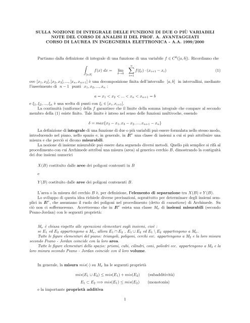
SULLA NOZIONE DI INTEGRALE DELLE FUNZIONI DI DUE O PIÙ VARIABILI
NOTE DEL CORSO DI ANALISI II DEL PROF. A. AVANTAGGIATI
CORSO DI LAUREA IN INGEGNERIA ELETTRONICA - A.A. 1999/2000
Partiamo dalla definizione di integrale di una funzione di una variabile f ∈ C 0 ([a, b]). Ricordiamo che
∫
[a,b]
f(x) dx =
lim
δ→0
n ∑
i=1
f(ξ i ) · (x i+1 − x i ) (1)
ove [x 1 , x 2 ], [x 2 , x 3 ], ..., [x n , x n+1 ] è una decomposizione finita dell’intervallo [a, b] in intervallini, mediante
l’inserimento di n − 1 punti x 1 , x 2 , ..., x n :
a = x 1 < x 2 < ... < x n < x n+1 = b
e ξ 1 , ξ 2 , ..., ξ n è una scelta di punti con ξ i ∈ [x i , x i+1 ].
La continuità (uniforme) della f garantisce che il limite della somma integrale che compare al secondo
membro della (1) esiste finito. Tale limite è inteso nel senso delle funzioni multivoche, essendo
δ = max{x 2 − x 1 , x 3 − x 2 , ..., x n+1 − x n }
La definizione di integrale di una funzione di due o più variabili può essere formulata nello stesso modo,
introducendo nel piano, nello spazio e, in generale, in IR ν una classe di insiemi a cui si può attribuire una
misura e che perciò si dicono misurabili.
La nozione di insieme misurabile può essere data seguendo diversi metodi. Quello più semplice si rifà al
procedimento con cui Archimede attribuì una misura (area) al generico cerchio B, dimostrando la contiguità
dei due insiemi numerici
X(B) costituito dalle aree dei poligoni contenuti in B
e
Y (B) costituito dalle aree dei poligoni contenenti B.
L’area o la misura del cerchio B è, per definizione, l’elemento di separazione tra X(B) e Y (B).
Lo sviluppo di questa idea richiede diverse precisazioni, soprattutto per determinare degli insiemi semplici
in IR ν , che assumano il ruolo dei poligoni nel procedimento (detto di esaustione) di Archimede. Su
ciò non ci soffermeremo. Accetteremo che in IR ν esista una classe M ν di insiemi misurabili (secondo
Peano-Jordan) con le seguenti proprietà:
M ν è chiusa rispetto alle operazioni elementari sugli insiemi, cioè :
se E 1 ed E 2 appartengono a M ν , allora E 1 ∩ E 2 , E 1 ∪ E 2 ed E 1 \ E 2 appartengono a M ν .
Tutte le figure elementari del piano: triangoli, poligoni, cerchi ecc. appartengono a M 2 e la loro misura
secondo Peano - Jordan coincide con la loro area.
Tutte le figure elementari dello spazio: prismi, cubi, cilindri, coni, poliedri ecc. appartengono a M 3 e la
loro misura secondo Peano - Jordan coincide con il loro volume.
In generale, la misura mis(·) su M ν ha le seguenti proprietà
e la importante proprietà additiva
mis(E 1 ∪ E 2 ) ≤ mis(E 1 ) + mis(E 2 )
E 1 ⊂ E 2 =⇒ mis(E 1 ) ≤ mis(E 2 )
(subadditività)
(monotonia)
1

Se E 1 ed E 2 non hanno punti interni in comune, allora
mis(E 1 ∪ E 2 ) = mis(E 1 ) + mis(E 2 ).
Gli insiemi misurabili più semplici che frequentemente intervengono nelle applicazioni sono:
I
Il rettangoloide di una funzione continua e non negativa f ∈ C 0 ([a, b]), così definito:
Per tale insieme è già noto che
C f = {(x, y) ∈ IR 2 | x ∈ [a, b] ; 0 ≤ y ≤ f(x)}
AreaC f = mis(C f ) =
∫ b
a
f(x) dx .
(cfr. [1], p. 232, Fig. 19)
II
Il dominio normale all’asse x determinato da due funzioni continue f(x) ≥ g(x) per x ∈ [a, b]
C f,g = {(x, y) ∈ IR 2 | x ∈ [a, b] ; g(x) ≤ y ≤ f(x)}
Per tale insieme è già noto che
AreaC f,g = mis(C f,g ) =
∫ b
a
[f(x) − g(x)] dx .
(cfr. [1], p. 232, Fig. 20)
2

III
Per l’analogo, normale all’asse y,
si ha ovviamente
C ′
l,h = {(x, y) ∈ IR 2 | y ∈ [c, d] ; h(y) ≤ x ≤ l(y)}
AreaC ′ f,g = mis(C ′ f,g) =
∫ d
c
[l(y) − h(y)] dy .
(cfr. [1], p. 232, Fig. 21)
È bene tener presente che, spesso, possono essere descritti con domini normali insiemi che apparentemente
non lo sono. Si fermi l’attenzione sul seguente esempio:
{(x, y) ∈ IR 2 | x 2 + (y − 1) 2 ≤ 4} = {(x, y) ∈ IR 2 | x ∈ [−2, 2] ; 1 − √ 4 − x 2 ≤ y ≤ 1 + √ 4 − x 2 }.
IV
(cfr. [1], p. 234, Fig. 23)
Il corrispettivo del rettangoloide in IR ν+1 si ottiene fissando una funzione f(P), definita, continua e non
negativa in un dominio limitato T di IR ν e ponendo ancora
C f = {(P, z) ∈ IR ν × IR | P ∈ T ; 0 ≤ z ≤ f(P)}.
Quando è ν > 1, C f si chiama cilindroide di base T relativo a f.
Nella teoria della misura secondo Peano-Jordan si dimostra:
3

Teorema (1): Se T è limitato e misurabile in IR ν ed f è continua in T , C f , come sottoinsieme di IR ν+1 ,
è misurabile, cioè C f ∈ M ν+1 .
In modo analogo si definiscono i domini normali in IR ν+1 .
V
(cfr. [1], p. 237, Fig. 26)
Siano f(x, y) e g(x, y) funzioni definite nel dominio T del piano 0xy; si introduce
C f,g = {(x, y, z) ∈ IR 3 | (x, y) ∈ T ; g(x, y) ≤ z ≤ f(x, y)}
Si dimostra:
Teorema (2): Se T è limitato e misurabile in IR 2 ( cioè T ∈ M 2 ) ed f, g ∈ C 0 (T ), allora C f,g ∈ M 3 .
VI
(cfr. [1], p. 232, Fig. 22)
Se f(x, y) e g(x, y) sono costanti in T ,
f(x, y) = d ; g(x, y) = c ∀(x, y) ∈ T
allora C f,g = T × [c, d] è un cilindro di sezione T .
Definizione di Integrale in IR ν
Fissata una f ∈ C 0 (T ), con T dominio limitato e misurabile di IR ν (T ∈ M ν ), si pone
∫
T
f(P) dT := lim
δ→0
n ∑
i=1
f(P i ) · mis(T i ) (2)
essendo {T 1 , ..., T n } una generica decomposizione finita di T in domini T 1 , ..., T n , tutti misurabili e a
due a due privi di punti interni in comune e quindi
T =
n⋃
T i e misT =
P 1 , ..., P n è una scelta di punti tali che P i ∈ T i , per i = 1, ..., n e
i=1
n∑
misT i ;
i=1
δ = max {diamT 1 , diamT 2 , ..., diamT n } .
Il limite al secondo membro della (2) è inteso nel senso delle funzioni multivoche ed esiste finito, a causa
della uniforme continuità della f in T .
Se f è costante ( f(P) = c ), si ha facilmente
∫
∫
f(P) dT = c dT = c · mis(T ) .
T
T
4

Fissate f e g ∈ C 0 (T ), si ha, per f ≥ 0,
∫
misC f = f(P) dT
e, per g ≤ f,
∫
misC f,g = [f(P) − g(P)] dT .
T
T
Bibliografia
[1] A. Avantaggiati - Analisi Matematica 2 - Ambrosiana Milano - 1995.
5