problemi ai limiti per equazioni differenziali ordinarie - Sezione di ...

Considereremo qui metodi numerici per la soluzione di problemi differenziali del secondoordine del tipoy ′′ = f(x,y,y ′ ), a < x < b, (1.1)con condizioni al bordoy(a) = α, y(b) = β. (1.2)Teorema 1.1. Assumiamo che f(x,y,z) soddisfi le ipotesi seguenti:i) f e le sue derivate parziali f y ≡ ∂f∂y e f z ≡ ∂f∂zsono continue in D = {(x,y,z)|a ≤ x ≤b, −∞ < y,z < ∞};ii) f y (x,y,z) > 0 in D;iii) esistono due costanti K e L tali cheK =max f y(x,y,z), L = max |f z(x,y,z)|.(x,y,z)∈D (x,y,z)∈DAllora la soluzione del problema differenziale ai limiti (1.1)-(1.2) esiste ed è unica.Se f(x,y,y ′ ) ha la formaf(x,y,y ′ ) = p(x)y ′ (x) + q(x)y(x) − r(x),il problema differenziale (1.1)-(1.2) si riduce al problema lineare⎧⎪⎨ y ′′ = p(x)y ′ + q(x)y − r(x), a < x < b,⎪⎩y(a) = α, y(b) = β.(1.3)Corollario 1.2. Assumiamo chei) p(x), q(x) e r(x) siano continue in [a,b];ii) q(x) > 0 per x ∈ [a,b].Allora, la soluzione del problema differenziale ai limiti (1.3) esiste ed è unica.Nel seguito faremo uso dell’operatore differenziale non lineareL y := −y ′′ + f(x,y,y ′ ), (1.4)e dell’operatore diffrenziale lineareK y := −y ′′ + p(x)y ′ + q(x)y . (1.5)Allora l’equazione differenziale (1.1) può essere scritta comeL y = 0. (1.6)mentre l’equazione differenziale lineare in (1.3) diventaK y = r(x). (1.7)2

2 Metodi alle differenze finiteI metodi alle differenze finite consistono nell’approssimare ciascuna derivata nelle equazioni differenziali(1.1) o (1.3) con una opportuna formula alle differenze finite.Prima di tutto introduciamo una discretizzazione dell’intervallo [a,b] dividendolo in N + 1sottointervalli uguali, cioè introduciamo i nodi equispaziatix i = a + ih, i = 0,1,... ,N + 1, h = b − aN + 1 . (2.1)Nei nodi interni x i , i = 1,... ,N, l’equazione differenziale (1.1) diventanel caso lineare, la (1.3) diventaL y(x i ) = −y ′′ (x i ) + f(x i ,y(x i ),y ′ (x i )) = 0; (2.2)L y(x i ) = −y ′′ (x i ) + p(x i )y ′ (x i ) + q(x i )y(x i ) = r(x i ). (2.3)Per risolvere numericamente i problemi differenziali (2.2) e (2.3) è necessario approssimaresia y ′ (x i ) che y ′′ (x i ). L’approssimazione viene scelta in modo che sia garantito uno specificoordine nell’errore di troncamento.Supponendo che y ∈ C 3 [x i−1 ,x i+1 ], si può ricorrere allo sviluppo in serie di Taylor di ordine2 per approssimare y(x i+1 ) e y(x i−1 ):y(x i+1 ) = y(x i + h) = y(x i ) + hy ′ (x i ) + 1 2! h2 y ′′ (x i ) + 1 3! h3 y ′′′ (η + i ),η + i ∈ (x i ,x i+1 ),y(x i−1 ) = y(x i − h) = y(x i ) − hy ′ (x i ) + 1 2! h2 y ′′ (x i ) − 1 3! h3 y ′′′ (η − i ),η − i ∈ (x i−1 ,x i ).Sottraendo la seconda equazione alla prima e usando il teorema della media si hay ′ (x i ) = y(x i+1) − y(x i−1 )2h− h26 y(3) (η i ), η i ∈ (x i−1 ,x i+1 ). (2.4)Questa è la formula alle differenze finite centrate per y ′ (x i ) e ha errore di troncamentoτ(x i ,y(x i );h;f) = − h26 y(3) (η i ) = O(h 2 ). (2.5)Per approssimare y ′′ (x i ) si utilizza lo sviluppo in serie di Taylor di ordine 3, purché y ∈3

C 4 [x i−1 ,x i+1 ]:y(x i+1 ) = y(x i + h) = y(x i ) + hy ′ (x i ) + 1 2! h2 y ′′ (x i ) + 1 3! h3 y ′′′ (x i )++ 1 4! h4 y (4) (ξ + i ), ξ+ i ∈ (x i ,x i+1 ),y(x i−1 ) = y(x i − h) = y(x i ) − hy ′ (x i ) + 1 2! h2 y ′′ (x i ) − 1 3! h3 y ′′′ (x i )++ 1 4! h4 y (4) (ξ − i ), ξ− i ∈ (x i−1 ,x i ).Sommando le due equazioni e usando il teorema della media si hay ′′ (x i ) = y(x i+1) − 2y(x i ) + y(x i−1 )h 2− h212 y(4) (ξ i ), ξ i ∈ (x i−1 ,x i+1 ). (2.6)Questa è la formula alle differenze finite centrate per y ′′ (x i ) e ha errore di troncamentoτ(x i ,y(x i );h;f) = − h212 y(4) (ξ i ) = O(h 2 ). (2.7)2.1 Metodo alle differenze finite non lineariSostituendo le formule alle differenze finite centrate (2.4) e (2.6) nell’equazione (2.2) si ha− y(x (i+1) − 2y(x i ) + y(x i−1 )h 2 +f x i ,y(x i ), y(x i+1) − y(x i−1 )−2h)− h26 y(3) (η i ) + h212 y(4) (ξ i ) = 0.Il metodo alle differenze finite non lineare si ottiene trascurando nella (2.8), che è una relazioneesatta, gli errori di troncamento (2.5) e (2.7), dovuti alle formule alle differenze finite, eaggiungendo le condizioni al bordo (1.2). Se con y i indichiamo l’approssimazione di y(x i ) si ha⎧⎪⎨⎪⎩y 0 = α, y N+1 = β,− y i+1 − 2y i + y i−1h 2(+ f x i ,y i , y )i+1 − y i−1= 0, i = 1,2,... ,N.2h(2.8)(2.9)4

Quindi, per trovare la soluzione approssimata {y i } N i=0 , si deve risolvere il sistema non lineare⎧(2y 1 − y 2 + h 2 f x 1 ,y 1 , y )2 − α− α = 0,2h⎪⎨⎪⎩(−y 1 + 2y 2 − y 3 + h 2 f x 2 ,y 2 , y )3 − y 1= 0,2h..........................................................................(−y N−2 + 2y N−1 − y N + h 2 f x N−1 ,y N−1 , y )N − y N−2= 0,2h(−y N−1 + 2y N + h 2 f x N ,y N , β − y )N−1− β = 0,2h(2.10)di N equazioni nelle N incognite y 1 ,y 2 ,...,y N .Prima di passare alla soluzione numerica del sistema non lineare (2.10) si deve verificare selo schema alle differenze finite costruito è convergente, cioè selim max |e i| = 0, (2.11)h→0 1≤i≤Ndove e i = |y(x i )−y i | è l’errore globale di troncamento. Come nel caso dei metodi per la soluzionedi problemi ai valori iniziali, la convergenza è assicurata se lo schema numerico è consistente estabile.Per studiare la consistenza e la stabilità dello schema alle differenze finite non lineare introduciamol’operatore differenziale discreto (non lineare) (L h y d ) i che agisce sulla funzione discretay d = {y i } N i=1 , associata alla discretizzazione (2.1), secondo lo schema alle differenze (2.9):(L h y d ) i := − y i+1 − 2y i + y i−1h 2(+ fx i ,y i , y i+1 − y i−12h). (2.12)Allora lo schema numerico (2.9) diventa⎧⎪⎨⎪⎩y 0 = α, y N+1 = β,(L h y d ) i = 0, i = 1,2,... ,N.(2.13)Tramite la soluzione esatta y(x) si può definire la funzione discreta y e := {y(x i )} N i=1 ; allora,(L h y e ) i = − y(x i+1) − 2y(x i ) + y(x i−1 )h 2(+ f x i ,y(x i ), y(x )i+1) − y(x i−1 )2hrappresenta l’operatore discreto che agisce sulla soluzione esatta.(2.14)5

Confrontando la (2.14) con la (2.8) si ha(L h y e ) i = −f(x i ,y(x i ), y(x i+1) − y(x i−1 )2h(+ f x i ,y(x i ), y(x )i+1) − y(x i−1 )=2h)− h26 y(3) (η i ) − h212 y(4) (ξ i )+(2.15)= f z (x i ,y(x i ),ζ i ) h26 y′′′ (η i ) − h212 y(4) (ξ i ),dove, nell’ultima uguaglianza, si è utilizzato lo sviluppo in serie di Taylor di(f x i ,y(x i ), y(x )i+1) − y(x i−1 )− h22h 6 y(3) (η i )nella terza variabile con punto iniziale y(x i+1) − y(x i−1 ); ζ i è un valore incognito compreso tra2hy ′ (x i ) = y(x i+1) − y(x i−1 )− h22h 6 y(3) (η i ) e y(x i+1) − y(x i−1 ).2hIn ciascun nodo, l’errore di troncamento dello schema numerico è definito come la differenzatra l’operatore differenziale esatto L y calcolato nel nodo x i e l’operatore differenziale discretoapplicato alla soluzione esatta (L h y e ) i :R(x i ,y(x i );h;f) = (L y)(x i ) − (L h y e ) i . (2.16)Utilizzando la relazione esatta (2.8), l’operatore differenziale esatto può essere scritto come(L y)(x i ) = −y ′′ (x i ) + f(x i ,y(x i ),y ′ (x i )) = − y(x i+1) − 2y(x i ) + y(x i−1 )h 2 ++f(x i ,y(x i ), y(x i+1) − y(x i−1 )2h)− h26 y′′′ (η i ) + h212 y(4) (ξ i ),(2.17)da cui segue che l’errore di troncamento valeR(x i ,y(x i );h;f) = −f z (x i ,y(x i ),ζ i ) h26 y′′′ (η i ) + h212 y(4) (ξ i ) = −(L h y e ) i , (2.18)dove η i e ξ i sono due punti incogniti nell’intervallo [x i−1 ,x i+1 ] e ζ i è , di nuovo, un valoreincognito compreso tra y ′ (x i ) = y(x i+1) − y(x i−1 )− h22h 6 y(3) (η i ) e y(x i+1) − y(x i−1 ).2hPoiché R(x i ,y(x i );h;f) = O(h 2 ), il metodo è consistente e del secondo ordine; inoltre èesatto per tutti i polinomi di grado ≤ 2.Per quanto riguarda la stabilità , nel caso di operatori discreti non lineari si può dare laseguente definizione.6

Definizione 2.1. Uno schema alle differenze finite non lineare è detto stabile se, date duefunzioni discrete v = {v i } N i=1 e u = {u i} N i=1 , definite sulla discretizzazione (2.1), esiste unacostante M tale che{max |v i − u i | ≤ M max(|v 0 − u 0 |, |v N+1 − u N+1 |)+0≤i≤N+1}+ max |(L h v) i − (L h u) i | .1≤i≤N(2.19)La stabilità è una proprietà dello schema numerico e rappresenta la capacità dello schemadi non amplificare ”troppo” le perturbazioni. Infatti, se con {y i } N i=1 indichiamo la soluzionedel problema discreto (2.13), e con {v i } N i=1 la soluzione di un problema discreto perturbato(L h v) i = ǫ i con condizioni al bordo v 0 = y(x 0 ) + ǫ 0 e v N+1 = y(x N+1 ) + ǫ N+1 , dalla disuguaglianza(2.19) si deduce che{}max |y i − v i | ≤ M max(|ǫ 0 |, |ǫ N+1 |) + max |ǫ i| , (2.20)0≤i≤N+1 1≤i≤Ncioè la perturbazione sulla soluzione si mantiene limitata.Per lo schema alle differenze finite non lineari vale il teorema seguente.Teorema 2.1. Siano L = max |f z(x,y,z)| e 0 < Q = min f y(x,y,z). Se hL ≤ 2, allora(x,y,z)∈D (x,y,z)∈Dlo schema alle differenze finite non lineari (2.13) è stabile con M = max(1,1/Q).La consistenza e la stabilità implicano la convergenza dello schema alle differenze finite.La stabilità fornisce anche una limitazione dell’errore globale. Infatti utilizzando nella disuguaglianza(2.19) le funzioni discrete {y(x i )} N i=1 e {y i} N i=1 e tenendo conto di (2.13) e (2.18) siottienemax |e i| = max |y(x i) − y i | ≤0≤i≤N+1 0≤i≤N+1≤ M max1≤i≤N |(L h y e ) i − (L h y d ) i | = M max1≤i≤N |R(x i,y(x i );h;f)|.(2.21)Infine, se valgono le ipotesi del Teorema 1.1 e se hL ≤ 2, il sistema non lineare (2.10) haun’unica soluzione.La soluzione discreta Y = [y 1 ,y 2 ,... ,y N ] T può essere approssimata con il metodo di Newtonche consiste nel generare una successione di approssimazioni {[y (k)1 ,y(k) 2 ,...,y(k) N ]T }, k = 1,2,....Se l’approssimazione iniziale [y (0)1 ,y(0) 2 , ...,y(0) N ]T è abbastanza vicina alla soluzione e la matriceJacobiana del sistema è regolare, allora la successione delle approssimazioni converge allasoluzione esatta.7

La matrice Jacobiana J(y 1 ,... ,y n ) del sistema (2.10) è tridiagonale con elementi⎧−1 + h (2 f z x i ,y i , y )i+1 − y i−1, j = i + 1,i = 1,... ,N − 1,2h(⎪⎨2 + h[J(y 1 ,... ,y n )] ij=2 f y x i ,y i , y )i+1 − y i−1, j = i,i = 1,... ,N,2h⎪⎩−1 − h 2 f z(x i ,y i , y i+1 − y i−12hdove y 0 = α e y N+1 = β.L’algoritmo del metodo di Newton è il seguente:), j = i − 1,i = 2,... ,N,⎧⎪⎨⎪⎩Y (0)datoJ(y (k)1 ,... ,y(k) n )V = B (k) ,Y (k+1) = Y (k) + V ,k = 0,1,... ,dove Y (k) = [y (k)1 ,y(k) 2 ,...,y(k) N ]T e[B (k) = −2y (k)1 − y (k)2 − α + h 2 f()x 1 ,y (k)1 , y(k) 2 − α,2h(−y (k)1 + 2y (k)2 − y (k)3 + h 2 f x 2 ,y (k)...,−y (k)N−2 + 2y(k) N−1 − y(k) N + h2 f2 , y(k)⎛3 − y (k) )1,...2h⎝x N−1 ,y (k)N−1 , y(k) N − y(k)2h⎞N−2⎠ ,−y (k)N−1 + 2y(k) N − β + h2 f⎛⎝x N ,y (k)N , β − y(k)2h⎞N−1⎠] T.Quindi ad ogni iterazione bisogna risolvere un sistema lineare tridiagonale, ad esempio con ilmetodo di Thomas che non ha un costo computazionale elevato.L’approssimazione iniziale Y (0) può essere ottenuta approssimando i valori y(x i ) con le ascissedella retta che congiunge i punti (a,α) e (b,β), cioè ponendoy (0)i= α + i( β − αb − a)h, i = 1,2,... ,N.Osserviamo che, anche se l’approssimazione può essere migliorata riducendo il passo h, nonconviene sceglierlo troppo piccolo a causa dell’instabilità che si produce nell’approssimare lederivate con le differenze finite.8

Esempio 2.1Consideriamo il problema ai limiti non lineare⎪⎨⎪⎩⎧⎪⎨⎪⎩y ′′ = 1 8 (32 + 2x3 − yy ′ ), 1 ≤ x ≤ 3,y(1) = 17, y(3) = 433 .Applicando il metodo alle differenze finite non lineare con passo h = 0.1 e nodi x i = 1.0 + ih,i = 0,1,... ,20, si ottiene il sistema non lineare⎧2y 1 − y 2 + h 21 ()32 + 2x 3 18− y y 2 − α1 − α = 0,2h−y 1 + 2y 2 − y 3 + h 21 8()32 + 2x 3 2 − y y 3 − y 12 = 0,2h..........................................................................−y N−2 + 2y N−1 − y N + h 21 8−y N−1 + 2y N + h 21 8()32 + 2x 3 N−1 − y y N − y N−2N−1 = 0,2h(32 + 2x 3 N − y N)β − y N−1− β = 0,2hla cui matrice Jacobiana è⎧−1 − h 2y i, i = j − 1,j = 2,... ,N,8⎪⎨[J(y 1 ,... ,y n )] ij=⎪⎩2 − h 2−1 + h 2y i+1 − y i−1, i = j,j = 1,... ,N,8y i, i = j + 1,j = 1,... ,N − 1.8Nella tabella di seguito è riportata la soluzione approssimata ottenuta con il metodo di Newtonutilizzando come criterio di arresto max 1≤x≤20 |y (k+1)i − y (k)i | ≤ 10 −8 ; per confronto è riportataanche la soluzione esatta.L’approssimazione può essere migliorata tramite l’estrapolazione di Richardson. Se con y (h)i indichiamol’approssimazione ottenuta con passo di integrazione h, l’estrapolazione di Richardson9

si applica avendo le tre approssimazioni con passo h, h/2 e h/4:Prima estrapolazione: y E 1iSeconda estrapolazione: y E 2i= 4y(h/2) i= 4y(h/4) i3− y (h)i− y (h/2)i3, i = 1,... ,N,, i = 1,... ,N,Estrapolazione finale: y E 3i = 16yE 2i − y E 1i, i = 1,... ,N.15Utilizzando come passo iniziale h = 0.1, l’approssimazione y E 3i ha un errore massimo di 3.68 ·10 −10 .i x i y i y(x i ) |y(x i ) − y i |0 1.0 17.000000 17.0000001 1.1 15.754503 15.755455 9.520×10 −42 1.2 14.771740 14.773333 1.594×10 −33 1.3 13.995677 13.997692 2.015×10 −34 1.4 13.386297 13.388571 2.275×10 −35 1.5 12.914252 12.916667 2.414×10 −36 1.6 12.557538 12.560000 2.462×10 −37 1.7 12.299326 12.301765 2.438×10 −38 1.8 12.126529 12.128889 2.360×10 −39 1.9 12.028814 12.031053 2.239×10 −310 2.0 11.997915 12.000000 2.085×10 −311 2.1 12.027142 12.029048 1.905×10 −312 2.2 12.111020 12.112727 1.707×10 −313 2.3 12.245025 12.246522 1.497×10 −314 2.4 12.425388 12.426667 1.278×10 −315 2.5 12.648944 12.650000 1.056×10 −316 2.6 12.913013 12.913846 8.335×10 −317 2.7 13.215312 13.215926 6.142×10 −418 2.8 13.553885 13.554286 4.006×10 −419 2.9 13.927046 13.927241 1.953×10 −420 3.0 14.333333 14.3333332.2 Metodo alle differenze finite lineariSostituendo le formule alle differenze finite centrate (2.4) e (2.6) nell’equazione lineare (2.3) siha− y(x i+1) − 2y(x i ) + y(x i−1 )h 2 +p(x i ) y(x i+1) − y(x i−1 )+ q(x i )y(x i )+2h(2.22)− h212 [2p(x i)y (3) (η i ) − y (4) (τ i )] = r(x i ),10

che da luogo allo schema alle differenze finite lineare⎧y ⎪⎨ 0 = α, y N+1 = β,⎪⎩− y i+1 − 2y i + y i−1h 2+ p(x i ) y i+1 − y i−12h+ q(x i )y i = r(x i ), i = 1,2,... ,N.In modo analogo a quanto fatto nel caso non lineare, definiamo l’operatore differenzialediscreto (lineare) che agisce sulla funzione discreta y d = {y i } N+1i=0 :(K h y d ) i = − y i+1 − 2y i + y i−1h 2cosicché lo schema numerico diventa⎧⎪⎨ y 0 = α, y N+1 = β,⎪⎩+ p(x i ) y i+1 − y i−12h(K h y d ) i = r(x i ), i = 1,2,... ,N.+ q(x i )y i , (2.23)(2.24)Se con (K h y e ) i indichiamo l’operatore discreto che agisce sulla soluzione esatta discretay e = {y(x i )} N+1i=0 , cioè(K h y e ) i = − y i+1 − 2y i + y i−1h 2= h212 [2p(x i)y (3) (η i ) − y (4) (ξ i )] ,+ p(x i ) y i+1 − y i−12hallora l’errore di troncamento dello schema numerico è dato daR(x i ,y(x i );h;f) = (K y)(x i ) − (K h y e ) i =+ q(x i )y i == − h212 [2p(x i)y ′′′ (η i ) − y (4) (ξ i )] = r(x i ) − (K h y e ) i .(2.25)(2.26)Poiché R(x i ,y(x i );h;f) = O(h 2 ), il metodo alle differenze finite lineare è consistente e delsecondo ordine; inoltre è esatto per tutti i polinomi di grado ≤ 2.Definizione 2.2. Uno schema alle differenze finite lineare è detto stabile se, data una funzionediscreta v = {v i } N+1i=0 , definita sulla discretizzazione (2.1), esiste una costante M tale che{}max |v i| ≤ M max (|v 0 |, |v N+1 |) + max |(K h v) i | . (2.27)0≤i≤N+1 1≤i≤NTeorema 2.2. Siano L = max |p(x)| e 0 < Q = min q(x). Se hL ≤ 2, allora lo schema allea≤x≤b a≤x≤bdifferenze finite lineari è stabile con M = max(1,1/Q).La consistenza e la stabilità implicano la convergenza dello schema lineare e inoltre per l’erroreglobale di troncamento si ha la limitazionemax |e i| = max |y(x i) − y i | ≤0≤i≤N+1 0≤i≤N+1≤ M max1≤i≤N |(K h y e ) i − (K h y d ) i | = M max1≤i≤N |R(x i,y(x i );h;f)|.(2.28)11

In questo caso la soluzione approssimata Y = [y 1 ,y 2 , · · · ,y N ] T si ottiene risolvendo il sistemalineare tridiagonale di N equazioni in N incognitedove⎡A =⎢⎣eAY = B,2 + h 2 q(x 1 ) −1 + h 2 p(x 1) 0 · · · · · · 0−1 − h 2 p(x 2) 2 + h 2 q(x 2 ) −1 + h 2 p(x 2) 0 · · · 0B =· · · · · · · · · · · · · · · · · ·0 · · · · · · −1 − h 2 p(x N−1) 2 + h 2 q(x N−1 ) −1 + h 2 p(x N−1)0 · · · · · · 0 −1 − h 2 p(x N) 2 + h 2 q(x N )[ (h 2 r(x 1 ) + 1 + h )(2 p(x 1) α, h 2 r(x 2 ), . . .,h 2 r(x N−1 ), h 2 r(x N ) + 1 − h ) T2 p(x N) β].⎤⎥⎦Se valgono le ipotesi del Teorema 2.2, il sistema tridiagonale ammette un’unica soluzione purchéh K ≤ 2.Esempio 2.2Consideriamo il problema ai limiti lineare⎧⎨y ′′ = 2⎩ x y′ − 2 sin(log x)x2y + , 1 ≤ x ≤ 2,xy(1) = 1, y(2) = 2,la cui soluzione esatta èy(x) = x ( )2 (4 − x) − x(1 − x) cos(log 2) + sin(log 2) − x22()cos(log x) + sin(log x) .Applicando il metodo alle differenze finite lineare si ottiene il sistema lineare tridiagonale⎡ (⎡⎤2 − h 2 2x 2 −1 + h 2h 2 sin(log x 1)+ 1 + h0 · · · · · · 0x2 x1 1 1 2−1 − h 22 − h 2 22 x 2 x 2 −1 + h 2h 2 sin(log x 2)0 · · · 0x2 x2 2 2X =· · · · · · · · · · · · · · · · · ·0 · · · · · · −1 − h 22 − h 2 2⎢2 x 8 x 2 −1 + h .22 x8 8h⎥2 sin(log x 8)x 8⎣⎦ ⎢⎣(0 · · · · · · 0 −1 − h 222 − h 2 2x 9 x 2 9h 2 sin(log x 9)x 9+1 − h 2)2αx 1)2βx 9⎤⎥⎦che può essere risolto con il metodo di Thomas. I risultati ottenuti sono riportati nella tabelladi seguito.Anche in questo caso si può utilizzare l’estrapolazione di Richardson per migliorare l’approssimazione.12

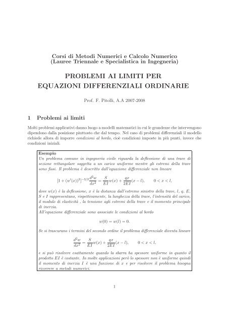
i x i y i y(x i ) |y i − y(x i )|0 1.0 1.00000000 1.000000001 1.1 1.08997132 1.09007246 1.01×10 −42 1.2 1.17916606 1.17935628 1.90×10 −43 1.3 1.26868985 1.26895130 2.61×10 −44 1.4 1.35967879 1.35998932 3.10×10 −45 1.5 1.45328006 1.45361424 3.34×10 −46 1.6 1.55063840 1.55096828 3.30×10 −47 1.7 1.65288668 1.65318237 2.96×10 −48 1.8 1.76113946 1.76136954 2.30×10 −49 1.9 1.87648855 1.87662038 1.32×10 −410 2.0 2.00000000 2.000000003 Metodi agli elementi finitiAbbiamo visto che nei metodi alle differenze finite si approssima la soluzione del problema ai limitisostituendo l’operatore di differenziazione continuo con un operatore discreto alle differenzefinite. I metodi agli elementi finiti seguono un approccio diverso. Per prima cosa il problemadifferenziale viene riscritto in forma variazionale in modo che la soluzione sia quella che minimizzaun opportuno operatore integrale (metodo di Rayleigh-Ritz) oppure quella che soddisfaun’equazione variazionale (metodo di Galerkin). La soluzione viene quindi approssimata conpolinomi a tratti, detti appunto elementi finiti, si cerca cioè un’approssimazione in uno spaziofunzionale di dimesione finita.Come problema modello, consideremo il problema differenziale lineare ai limiti⎧⎪⎨⎪⎩− d (dxp(x) dydxy(0) = y(1) = 0,)+ q(x)y = f(x), 0 < x < 1,che descrive la deflessione y(x) di una sbarra sottile di lunghezza 1 con sezione variabile q(x).La deflessione è dovuta alle forze esterne p(x) e f(x).Assumeremo che p ∈ C 1 ([0,1]) e q, f ∈ C([0,1]) e che esista una costante δ tale chep(x) ≥ δ > 0 e che q(x) ≥ 0 per x ∈ [0,1].Queste condizioni sono sufficienti a garantire che il problema differenziale ai limiti (3.1) abbiaun’unica soluzione y ∈ C0 2 ([0,1]), doveC 2 0([0,1]) = {u ∈ C 2 ([0,1]);u(0) = u(1) = 0}.Come succede in molti problemi ai limiti che descrivono fenomeni fisici, la soluzione dell’equazionedella sbarra soddisfa principi variazionali, che possono essere la minimizzazione di un funzionaledell’energia oppure il principio dei lavori virtuali.(3.1)13

Teorema 3.1. Siano p ∈ C 1 ([0,1]), q e f ∈ C([0,1]) ed esista una costante δ > 0 tale chep(x) ≥ δ e, inoltre, q(x) ≥ 0 per x ∈ [0,1]. La funzione y ∈ C0 2 ([0,1]) è l’unica soluzionedell’equazione differenziale− d (p(x) dy )+ q(x)y = f(x), 0 < x < 1, (3.2)dx dxcon condizioni al bordoy(0) = y(1) = 0, (3.3)se e solo se è l’unica funzione in C0 2 ([0,1]) che minimizza l’integraleI[u] =∫ 10o, equivalentemente, che soddisfa l’equazione variazionale∫ 10dove u ∈ C 1 ([0,1]) con u(0) = u(1) = 0.{}p(x)[u ′ (x)] 2 + q(x)[u(x)] 2 − 2f(x)u(x) dx. (3.4){}p(x)y ′ (x)u ′ (x) + q(x)y(x)u(x) dx =∫ 10f(x)u(x)dx, (3.5)L’integrale I[u] rappresenta l’energia del sistema, quindi la soluzione y è quella che minimizzal’energia; la forma variazionale (3.5) invece è il principio dei lavori virtuali.Quando la soluzione y è sufficientemente regolare, allora le tre formulazioni del problemasono equivalenti e si può scegliere quella che si ritiene più conveniente dal punto di vistanumerico. Poichè la regolarità della soluzione dipende dal dato f, è sufficiente che f siacontinua perché y ∈ C 2 ([0,1]).D’altra parte, la formulazione variazionale, sia in termini di energia che attraverso il principiodei lavori virtuali, ha senso anche quando il dato f è meno regolare (per esempio, costantea tratti oppure concentrato in alcuni punti): in questi casi il problema fisico viene formulatodirettamente nella forma variazionale, mentre la forma differenziale perde di significato. Osserviamoche le formulazioni variazionali (3.4) e (3.5) sono definite sotto ipotesi meno restrittivesulla y, infatti è sufficiente che y ∈ C 0 ([0,1]) e y ′ sia continua a tratti perchè gli integrali abbianosenso.La soluzione del problema differenziale (3.1) appartiene allo spazio di dimensione infinitaC 2 0 ([0,1]). Nel metodo degli elementi finiti si approssima la soluzione in uno spazio V N di dimesionefinita N. Se le funzioni {ψ 1 ,ψ 2 ,... ,ψ N } formano una base in V N , l’approssimazione y Ndi V N può essere scritta nella formay N (x) = γ 1 ψ 1 (x) + γ 2 ψ 2 (x) + · · · γ N ψ N (x).Le funzioni ψ j , j = 1,2,... ,N, sono chiamate funzioni prova (trial functions), e sono usualmentefamiglie di polinomi ortogonali (Chebyshev, Legendre, Lagrange), funzioni splines oppurefunzioni trigonometriche. I parametri γ j , j = 1,2,... ,N, detti gradi di libertà , sono le incognitedel problema.I coefficienti incogniti γ j , j = 1,2,... ,N, vengono determinati imponendo che y N soddisfi ilprincipio del minimo dell’energia (metodo di Rayleigh-Ritz) oppure il principio dei lavori virtuali(metodo di Galerkin).14

3.1 Metodo di Rayleigh-RitzNel metodo di Rayleigh-Ritz le incognite γ j , j = 1,... ,N, vengono determinate minimizzandol’integrale (3.4) non su tutte le funzioni u ∈ C0 2 ([0,1]), ma sull’insieme più piccolo di funzioni cheappartengono allo spazio V N . In altre parole, l’approssimazione [ y N (x) di y si ottiene trovando∑Nj=1 ]i valori di γ j , j = 1,... ,N, che minimizzano l’integrale I γ j ψ j .Dall’equazione (3.4) si ha⎡ ⎤N∑I[y N ] = I ⎣ γ j ψ j⎦ ==j=1 ⎧∫ 10⎡⎪⎨⎪⎩ p(x) ⎣⎤2⎡ ⎤2⎡ ⎤⎫N∑N∑N∑⎪⎬γ j ψ j ′(x) ⎦ + q(x) ⎣ γ j ψ j (x) ⎦ − 2f(x) ⎣ γ j ψ j (x) ⎦j=1j=1j=1⎪⎭ dx.Affinché I, come funzione di γ 1 ,... ,γ N , abbia un minimo deve essere∂I∂γ k= 0,k = 1,2,... ,N,quindi∂I∂γ k=⎧∫ 1 ⎨0⎫N⎩ 2p(x) ∑N γ j ψ j ′(x)ψ′ k (x) + 2q(x) ∑⎬γ j ψ j (x)ψ k (x) − 2f(x)ψ k (x) dx = 0,⎭j=1j=1k = 1,2,... ,N.Le equazioni precedenti formano un sistema lineare di N equazioni nelle N incognite Γ =[γ 1 ,...,γ N ] T . La matrice dei coefficienti A, chiamata matrice di rigidità (stiffness matrix), èsimmetrica e ha elementia jk =∫ 10{}p(x)ψ j(x)ψ ′ k(x) ′ + q(x)ψ j (x)ψ k (x) dx; (3.6)il termine noto F, chiamato vettore di carico (load vector), ha elementi3.2 Elementi finiti linearif k =∫ 10f(x)ψ k (x)dx. (3.7)Nel metodo degli elementi finiti lineari si sceglie come spazio di funzioni approssimanti V N lospazio delle funzioni spline lineari nell’intervallo [0,1] che assumono valore nullo agli estremidell’intervallo.Sia ∆ : 0 = x 0 < x 1 < x 2 < ... < x N < x N+1 = 1 una partizione dell’intervallo [0,1] e siah i = x i − x i−1 , i = 1,2,... ,N + 1, allora V N è lo spazio dei polinomi lineari a tratti in [0,1] conderivata discontinua nei nodi x i , i = 1,2,... ,N, e che assumono valore 0 in x 0 = 0 e x N+1 = 1.15

Le funzioni di base ψ j , j = 1,2,... ,N, per lo spazio V N , sono i polinomi lineari a trattidefiniti dalle proprietà di interpolazioneda cui si ottiene⎧⎪⎨ψ j (x) =⎪⎩ψ j (x i ) ={1, se i = j,0, se i ≠ j,x − x j−1h j, se x ∈ [x j−1 ,x j ],x j+1 − xh j+1, se x ∈ [x j ,x j+1 ],0, altrove,(3.8)j = 1,... ,N. (3.9)Le derivate delle funzioni ψ j sono costanti nei sottointervalli (x j ,x j+1 ), j = 0,1,... ,N, esono date da⎧1, se x ∈ (x j−1 ,x j ),⎪⎨ h jψ j(x) ′ =− 1 , se x ∈ (x j ,x j+1 ),j = 1,... ,N. (3.10)h ⎪⎩ j+10, altrove.L’approssimazione della soluzione y(x) nello spazio a dimensione finita V N generato dallabase di funzioni ψ j , j = 1,2,... ,N, èN∑y N (x) = γ j ψ j (x), x ∈ [0,1]. (3.11)j=1Ovviamente in questo caso y N è un polinomio lineare a tratti, cioè y N (x) ∈ C 0 ([0,1]) e y N ′ ècontinua a tratti, con y N (0) = y N (1) = 0; inoltre, y N (x i ) = γ i , i = 1,2,... ,N.Utilizzando nelle formule (3.6) e (3.7) le espressioni di ψ j e ψ j ′ date in (3.9) e (3.10) si haa kk =∫ 10{p(x)[ψ ′ k (x)]2 + q(x)[ψ k (x)] 2} dx =( ) 1 2 ∫ xk( ) 1 2 ∫ xk+1= p(x)dx +p(x)dx+h k x k−1h k+1( ) 1 2 ∫ xk( ) 1 2 ∫ xk+1+ (x − x k−1 ) 2 q(x)dx +(x k+1 − x) 2 q(x)dxh k x k−1h k+1x kx kk = 1,2,... ,N16

a k,k+1 =∫ 10{}p(x)ψ k ′ (x)ψ′ k+1 (x) + q(x)ψ k(x)ψ k+1 (x) dx =( ) 1 2 ∫ xk+1( ) 1 2 ∫ xk+1= −p(x)dx +(x k+1 − x)(x − x k )q(x)dxh k+1 x kh k+1x kk = 1,2,... ,N − 1a k,k−1 =f k =∫ 10∫ 10{}p(x)ψk ′ (x)ψ′ k−1 (x) + q(x)ψ k(x)ψ k−1 (x) dx =( ) 1 2 ∫ xk( ) 1 2 ∫ xk= − p(x)dx + (x k − x)(x − x k−1 )q(x)dxh k x k−1h k x k−1f(x)ψ k (x)dx == 1 ∫ xk(x − x k−1 )f(x)dx + 1 ∫ xk+1h k x k−1h k+1k = 2,... ,Nx k(x k+1 − x)f(x)dx k = 1,2,... ,N.Osserviamo che la matrice A è tridiagonale poiché ciascuna funzione ψ j , j = 1,2,... ,N, èdiversa da zero solo nell’intervallo (x j−1 ,x j+1 ) e quindi si sovrappone solo alle funzioni ψ j−1 eψ j+1 .Ci sono sei tipi di integrali da calcolare. DefinendoQ 1,k =1(h k+1 ) 2 ∫ xk+1x k(x k+1 − x)(x − x k )q(x)dx, k = 1,2,... ,N − 1,Q 2,k = 1(h k ) 2 ∫ xkx k−1(x − x k−1 ) 2 q(x)dx,k = 1,2,... ,N,Q 3,k =1(h k+1 ) 2 ∫ xk+1x k(x k+1 − x) 2 q(x)dx, k = 1,2,... ,N,Q 4,k = 1(h k ) 2 ∫ xkx k−1p(x)dx, k = 1,2,... ,N + 1,Q 5,k = 1 h k∫ xkx k−1(x − x k−1 )f(x)dx,k = 1,2,... ,N,Q 6,k = 1h k+1∫ xk+1x k(x k+1 − x)f(x)dx, k = 1,2,... ,N,17

si possono scrivere gli elementi della matrice di rigidità A e del vettore di carico F in modo piùcompatto:a k,k = Q 4,k + Q 4,k+1 + Q 2,k + Q 3,k , k = 1,2,... ,N,a k,k+1 = −Q 4,k+1 + Q 1,k , k = 1,2,... ,N − 1,a k,k−1 = −Q 4,k + Q 1,k−1 ,k = 2,3,... ,N,f k = Q 5,k + Q 6,k ,k = 1,2,... ,N.Risolvendo il sistema lineare AΓ = F si trovano le incognite Γ che permettono di costruirel’approssimazione y N .Si può dimostrare che la matrice tridiagonale A è simmetrica e definita positiva quindi ilsistema lineare ammette un’unica soluzione ed è anche ben condizionato. Inoltre, sotto le ipotesisu p, q, e f date nel Teorema 3.1, si hamaxx∈[0,1] |y(x) − y N(x)| = O(h 2 ), x ∈ [0,1],quindi il metodo è convergente e del secondo ordine.La difficoltà di questo metodo sta nel dover valutare i 6n integrali Q j,k , che possono esserecalcolati direttamente solo in casi elementari. In generale bisogna ricorrere a una formula diquadratura oppure si possono approssimare le funzioni p, q e f con un polinomio lineare a trattie integrare poi tale polinomio.Per ottenere funzioni approssimanti più regolari si può approssimare la soluzione y(x) confunzioni splines di ordine più elevato; ad esempio, se si usano le spline cubiche l’approssimantey N è in C0 2 ([0,1]), però in questo caso le funzioni di base hanno un supporto più ampio e lamatrice di rigidità è pentadiagonale. Come conseguenza aumenta il costo computazionale siadella costruzione della matrice di rigidità , che è meno sparsa, sia della soluzione del sistemalineare.Esempio 3.1Consideriamo il problema ai limiti{−y ′′ + π 2 y = 2π sin(πx), 0 ≤ x ≤ 1,y(0) = y(1) = 0.Per approssimare la soluzione introduciamo una partizione di 10 nodi equispaziati con passoh k = h = 0.1, quindi x k = 0.1k, k = 0,1,... ,10. In questo caso gli integrali Q j,k possono essere18

calcolati esattamente:Q 1,k = 100∫ 0.1k+0.10.1k(0.1k + 0.1 − x)(x − 0.1k)π 2 dx = π260 ,∫ 0.1kQ 2,k = 100 (x − 0.1k + 0.1) 2 π 2 dx = π20.1k−0.130 ,∫ 0.1k+0.1Q 3,k = 100 (0.1k + 0.1 − x) 2 π 2 dx = π20.1k30 ,∫ 0.1kQ 4,k = 100 dx = 10,0.1k−0.1∫ 0.1kQ 5,k = 10 (x − 0.1k + 0.1)2π 2 sin(πx)dx =0.1k−0.1= −2π cos(0.1πk) + 20[sin(0.1πk) − sin(0.1k − 0.1)π)],∫ 0.1k+0.1Q 6,k = 10 (0.1k + 0.1 − x)2π 2 sin(πx)dx =0.1k= 2π cos(0.1πk) − 20[sin(0.1k + 0.1)π) − sin(0.1πk)].Gli elementi di A e F sono dati daLa soluzione del sistema tridiagonale èa k,k = 20 + π2, k = 1,2,... ,9,15a k,k+1 = −10 + π2, k = 1,2,... ,8,60a k,k−1 = −10 + π2, k = 2,3,... ,9,60f k = 40sin(0.1πk)[1 − cos(0.1π)], k = 1,2,... ,9.γ 9 = 0.31029, γ 8 = 0.59020, γ 7 = 0.81234,γ 6 = 0.95496, γ 5 = 1.00411, γ 4 = 0.95496,γ 3 = 0.81234, γ 2 = 0.59020, γ 1 = 0.31029.L’approssimazione polinomiale a tratti della soluzione èy 9 (x) =9∑γ k ψ k (x),k=119

mentre la soluzione esatta è data da y(x) = sin(πx). In tabella sono riportati i valori numericie l’errore.i x i y(x i ) y 9 (x i ) = γ i |y(x i ) − γ i |1 0.1 0.30902 0.31029 0.001272 0.2 0.58779 0.59020 0.002413 0.3 0.80902 0.81234 0.003324 0.4 0.95106 0.95496 0.003905 0.5 1.00000 1.00411 0.004116 0.6 0.95106 0.95496 0.003907 0.7 0.80902 0.81234 0.003328 0.8 0.58779 0.59020 0.002419 0.9 0.30902 0.31029 0.001273.3 Metodo di GalerkinIn questo metodo i coefficienti incogniti γ j , j = 1,2,... ,N, vengono determinati imponendoche y N soddisfi il principio dei lavori virtuali (3.5). Questo vuol dire che y N deve soddisfare ilseguente problema discreto∫ 10{} ∫ 1p(x)y N ′ (x)u′ N (x) + q(x)y N(x)u N (x) dx = f(x)u N (x)dx) (3.12)0per ogni u N ∈ V N . Sostituendo nella (3.12) l’espressioni di y N data in (3.11) e ponendoN∑u N (x) = c j ψ j (x), x ∈ [0,1],j=1si ottiene un sistema lineare che, a causa della simmetria dell’equazione variazionale, coincidecon quello che si ottiene con il metodo di Rayleigh-Ritz. Allora la soluzione del sistema è unicae quindi esiste un’unica approssimazione y N della soluzione del principio dei lavori virtuali.Per quanto riguarda la convergenza e l’ordine valgono considerazioni analoghe a quelle fatteper il metodo di Rayleigh-Ritz.4 Metodo di Newton per sistemi non lineariConsideriamo il sistema non lineareF(X) = 0 (4.13)con X = [x 1 ,x 2 ,...,x n ] T e F(X) = [f 1 (X),f 2 (X),... ,f n (X)] T . Una soluzione del sistema(4.13) è un vettore ¯X = [¯x 1 , ¯x 2 ,... , ¯x n ] T tale cheF( ¯X) = 0.Se le funzioni f 1 (x 1 ,... ,x n ),... ,f n (x 1 ,... ,x n ), ammettono derivate parziali limitate, allora lasoluzione ¯X può essere approssimata con il metodo di Newton. Partendo da una approssimazione20

iniziale X (0) = [x (0)1 ,x(0) 2 ,... ,x(0) n ] T , si costruisce una successione di approssimazioni {X (k) =[x (k)1 ,x(k) 2 ,...,x(k) n ] T }, k = 1,2,..., con un procedimento iterativo del tipo{X(0)dato,X (k) = X (k−1) − J(X (k−1) ) −1 F(X (k−1) ), k ≥ 1,dove J(X) è la matrice Jacobiana del sistema (4.13). Se l’approssimazione iniziale è sufficientementeaccurata e lo Jacobiano è regolare il metodo è convergente, cioèlimk→∞ X(k) = ¯X ⇔e la convergenza è quadratica quindilim || ¯X − X (k) || = 0,k→∞||lim¯X − X (k+1) ||k→∞ || ¯X − X (k) || 2 = C,dove C è una costante positiva.La difficoltà del metodo di Newton consiste nel fatto che ad ogni passo bisogna invertirela matrice Jacobiana che richiede un costo computazionale elevato. Per evitare l’inversione dimatrice si procede nel modo seguente. Ad ogni passo si risolve il sistema lineareJ(X (k−1) )Y = −F(X (k−1) )quindi si calcola la nuova approssimazione X (k) = X (k−1) + Y . Il procedimento iterativo vienearrestato quando ||X (k) − X (k−1) || ≤ ǫ, dove ǫ è una tolleranza prefissata.Bibliografia1. R.L. Burden, J.D. Faires, Numerical Analysis, Books/Cole Pubbling Company, 1997(§§ 11.3-11.5).2. V. Comincioli, Analisi Numerica. Metodi, Modelli e Applicazioni, McGraw-Hill, 1990(§§ 9.5.2-9.5.3).3. W. Gautschi, Numerical Analysis, Birkhauser, 1997 (§§ 6.1, 6.3, 6.4).4. L. Gori, Calcolo Numerico, Ed. Kappa, 1999 (§§ 6.15, 9.13).5. L. Gori, Soluzione Numerica di Problemi alle Derivate Parziali. Metodi alle DifferenzeFinite, Dispense, 2001 (§ 3).6. G. Strang, G.J. Fix, An Analysis of the Finite Element Method, Prentice-Hall, 1973.21