OPTIMIZATION PROBLEMS IN MASS TRANSPORTATION THEORY ...

OPTIMIZATION PROBLEMS INMASS TRANSPORTATION THEORYGiuseppe ButtazzoDipartimento di MatematicaUniversità di Pisabuttazzo@dm.unipi.ithttp://cvgmt.sns.itSchool on Calculus of VariationsRoma July 4–8, 2005

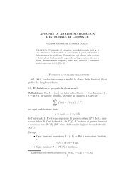
Mass transportation theory goes back toGaspard Monge (1781) when he presented amodel in a paper on Académie de Sciencesde Parisremblais•T(x)déblais•xThe elementary work to move a particle xinto T (x) is given by |x − T (x)|, so that thetotal work is∫|x − T (x)| dx .déblaisA map T is called admissible transport mapif it maps “déblais” into “remblais”.1

The Monge problem is thenmin{ ∫ déblais |x − T (x)| dx : T admiss. }.It is convenient to consider the Monge problemin the framework of metric spaces:• (X, d) is a metric space;• f + , f − are two probabilities on X(f + = “déblais”, f − = “remblais”);• T is an admissible transport map ifT # f + = f − .The Monge problem is then{ ∫minXd ( x, T (x) ) }dx : T admiss. .In general the problem above does not admita solution, when the measures f + andf − are singular, since the class of admissibletransport maps can be empty.2

Example Take the measuresf + = δ A and f − = 1 2 δ B + 1 2 δ C ;it is clear that no map T transports f + intof −so the Monge formulation above is inthis case meaningless.Example Take the measures in R 2 , still singularbut nonatomicf + = H 1 ⌊A and f − = 1 2 H1 ⌊B + 1 2 H1 ⌊Cwhere A, B, C are the segments below.CAB3

Then the class of admissible transport mapsis nonempty but the minimum in the Mongeproblem is not attained. Indeed, if the distancebetween the lines is L and the heightis H it can be seen that the infimum of theMonge cost is HL, while every transportmap T has a cost strictly greater than HL.Example (book shifting) Consider in R themeasuresf + = 1 [0,a] L 1 , f − = 1 [b,a+b] L 1 .Then the two mapsT 1 (x) = b + x,T 2 (x) = a + b − xare both optimal; the map T 1 corresponds toa translation, while the map T 2 correspondsto a reflection. Indeed there are infinitelymany optimal transport maps.4

Example TakeN∑N∑f + = δ pi f − = δ ni .i=1i=1Then the optimal Monge cost is given by theminimal connection of the p i with the n i .Relaxed formulation (due to Kantorovich):consider measures γ on X × X• γ is an admissible transport plan ifπ # 1 γ = f + and π # 2 γ = f − .• Transport plans γ that are concentratedon γ-measurable graphs are actually transportmaps T : X → X, via the equalityγ = (Id × T ) # f + .5

Monge-Kantorovich problem:{ ∫ }min d(x, y) dγ(x, y) : γ admiss. .X×XTheorem There exists an optimal transportplan γ opt ; in the Euclidean case γ optis actually a transport map T opt wheneverf + and f − are in L 1 .The existence part is easy; indeed in thecase X compact it follows from the weak*compactness of probabilities and the weak*continuity of the Monge-Kantorovich cost.In the general case the same holds by usingthe boundedness of the first moments.Note that, while in the Monge problem thecost is highly nonlinear with respect to theunknown T , in the Kantorovich formulationthe cost is linear with respect to the unknownγ.6

The Kantorovich formulation can be seenas the relaxation of the Monge problem; indeed,if f + is nonatomic we havemin(Kantorovich) = inf(Monge).The existence of an optimal transport mapis a rather delicate question. The first (incomplete)proof is due to Sudakov (1979);various different proofs have been givenby Evans-Gangbo (1999), Trudinger-Wang(2001), Caffarelli-Feldman-McCann (2002),Ambrosio (2003).Wasserstein distance of exponent p: replace( ∫ ) 1/p.the cost byX×X dp (x, y) dγ(x, y)Most of the results remain valid for moregeneral cost functions c(x, y).7

Shape optimization problemsThere is a strong link between mass transportationand shape optimization problems.We present here this relation and we refer tothe papers by Bouchitté-Buttazzo [BB] andBouchitté-Buttazzo-Seppecher [BBS] for alldetails.Shape optimization problem in elasticity:given a force field f in R n find the elasticbody Ω whose “resistance” to f is maximalConstraints:- given volume, |Ω| = m- possible “design region” D given, Ω ⊂ D- possible support region Σ given,Dirichlet regionOptimization criterion: elastic compliance8

More precisely, for every admissible domainΩ we consider the energy{ ∫E(Ω) = inf j(Du) dx − 〈f, u〉 :Ω}u smooth, u = 0 on Σand the elastic complianceC(Ω) = −E(Ω).In the linear case, when j is a quadraticform, an integration by parts gives that theelastic compliance reduces to the work ofexternal forcesC(Ω) = 1 2 〈f, u Ω〉being u Ω the displacement of minimal energyin Ω. In linear elasticity, if z ∗ = sym(z)and α, β are the Lamé constants,j(z) = β|z ∗ | 2 + α 2 |trz∗ | 2 .9

The shape optimization problem above hasin general no solution; in fact minimizing sequencesmay develop wild oscillations whichgive raise to limit configurations that are notin a form of a domain.Therefore, in order to describe the behaviourof minimizing sequences a relaxedformulation is needed.The literature on this problem is very wide;starting from the works by Murat and Tartarin the ’70, it has been studied bymany authors (Kohn and Strang, Lurie andCherkaev, Allaire, Bendsøe, . . . ). There arestrong links with homogenization theory.A large parallel literature is present in engineering.11

The complete relaxed form of the problemabove is not known: several difficulties arise.For instance:• Lack of coercivity; in most of the literaturemixtures of two homogeneous isotropicmaterials are considered. Hereone of the two materials is the emptyspace (outside Ω).• Even for mixtures of two materials in theelasticity case the set of materials attainableby relaxation is not known.• Possibility of nonlocal problems as limitsof admissible sequences of domains.• When D is unbounded, it is not clearthat data with compact support provideminimizing sequences of domains thatare equi-bounded.12

To overcome some of these difficulties it isconvenient to study a slightly different problemwhere we have the freedom to distributea given quantity of material without the restrictionof designing a domain Ω. They arecalled Mass Optimization Problems andconsist in finding, given a force field f in R n(which may possibly concentrate on sets oflower dimension), the mass distribution µwhose “resistance” to f is maximal.Constraints:• given mass, ∫ dµ = m• possible design region D given,with spt µ ⊂ D• possible support region Σ given,Dirichlet region.13

Optimization criterium:elastic complianceAs before for every admissible mass distributionµ we consider the energy{ ∫E(µ) = inf j(Du) dµ − 〈f, u〉 :}u smooth, u = 0 on Σand the elastic compliance C(µ) = −E(µ).Then the mass optimization problem is{∫ }min C(µ) : spt µ ⊂ D, dµ = m .Elasticity: u and f vector-valued,j(z) = β|z ∗ | 2 + α 2 |trz∗ | 2 .Conductivity: u and f scalar,j(z) = 1 2 |z|2 .14

In the mass optimization problem there ismore freedom than in the shape optimizationproblem because we may use measuresdifferent from µ = 1 Ω dx, as it occurs inshape optimization problems.On the other hand, we are not restrictedonly to forces in H −1 or to n or n−1 dimensionalDirichlet regions; for instance we mayconsider forces and Dirichlet regions concentratedin a single point, or in a finite numberof points.Of course, for a given f, we may haveE(µ) = −∞ for some measures µ; for instancethis occurs when f is a Dirac massand µ is the Lebesgue measure on a domainΩ, but these measures with infinite complianceare ruled out by the optimization criterionwhich consists in maximizing E(µ).15

There is a strong link between the mass optimizationproblem and the Monge-Kantorovichmass transfer problem.This is described below in the scalar case,the elasticity case being still not completelyunderstood.When in the mass optimization problem wehave Σ = ∅ and D = R n , then the associateddistance in the transportation problemis the Euclidean one.On the contrary, if a Dirichlet region Σ anddesign region D are present, the Euclideandistance |x − y| has to be replaced by anotherdistance d(x, y) which measures thegeodesic distance in D between the points xand y, counting for free the paths along Σ.16

More precisely, we consider the geodesic distanceon D × D{ ∫ 1d D (x, y) = min |γ ′ (t)| dt :0}γ(t) ∈ D, γ(0) = x, γ(1) = y= sup { |ϕ(x) − ϕ(y)| :|Dϕ| ≤ 1 on D }and its modification by Σ{d D,Σ (x, y) = inf d D (x, y) ∧ ( d D (x, ξ 1 )+ d D (y, ξ 2 ) ) }: ξ 1 , ξ 2 ∈ Σ= sup { |ϕ(x) − ϕ(y)| :|Dϕ| ≤ 1 on Ω, ϕ = 0 on Σ } .This semi-distance will play the role of costfunction in the Monge-Kantorovich masstransport problem.17

When f = f + − f − is a smooth function,D = R n , Σ = ∅, Evans and Gangbo [Mem.AMS 1999] have shown that the solution canbe found by solving the PDE⎧⎨ − div ( a(x)Du ) = fu is 1-Lipschitz⎩|Du| = 1 a.e. on {a(x) > 0}where the coefficient a is a multiple of theoptimal µ.However, even simple cases with f ∈ H −1may produce optimal mass distributionswhich are singular measures. For instancef +f - 18

produces an optimal µ which has a onedimensionalconcentration in the vertical segment.Then a theory of variational problems withrespect to measures has to be developed.This has been done by Bouchitté, Buttazzoand Seppecher [Calc. Var. 1997]. The applicationof transport problems to mass optimizationhas been developed by Bouchittéand Buttazzo [JEMS 2001]. The key toolsare:• the tangent space T µ (x) to a measure µ,defined for µ a.e. x;• the tangential gradient D µ ;• the Sobolev spaces W 1,pµ .19

Then the transport problem becomes equivalentto the PDE⎧⎨ − div ( µ(x)D µ u ) = f in R n \ Σu is 1-Lipschitz on D, u = 0 on Σ⎩|D µ u| = 1 µ-a.e. on R n , µ(Σ) = 0.Theorem. For every measure f thereexists a solution µ opt of the mass optimizationproblem. Moreover, a measure µsolves the mass optimization problem if andonly if (a multiple of) it solves the Monge-Kantorovich PDE.In order to describe the tangential gradientsD µ u which appear in the Monge-Kantorovich equation above we recall themain steps of the theory of the variationalintegrals w.r.t. a measure.20

Variational integrals w.r.t. a measureConsider the functional∫F (u) = f(x, Du) dµdefined for smooth functions u (and +∞elsewhere), where µ is a general nonnegativemeasure.On the integrand f we assumethe usual convexity and p-growth conditions.We define the tangent fieldsX p′µ = { φ ∈ L p′µ (R n ; R n ) :the tangent spacesdiv(φµ) ∈ L p′µ (R n ) } ,T p µ(x) = µ-ess ⋃ {φ(x) : φ ∈ Xp ′µthe tangential gradient (for smooth functions)D µ u(x) = P µ (x, Du(x)).},21

The operator D µ is closable, i.e.{uh → 0 weakly in L p µD µ u h → v weakly in L p ⇒ v = 0 µa.e.µand we still denote by D µ its closure. TheSobolev space W 1,pµ is then defined as thedomain of the extension above, with norm‖u‖ 1,p,µ = ‖u‖ Lpµ+ ‖D µ u‖ Lpµ.The relaxation of the integral functionalabove is given by∫F (u) = f µ (x, D µ u) dµ u ∈ Wµ1,pwheref µ (x, z) = inf { f(x, z+ξ) : ξ ∈ ( T p µ(x) ) ⊥}.In particular,∫|Du| 2 dµrelaxes to∫|D µ u| 2 dµ .22

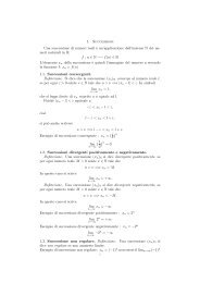
Here are some cases where the optimal massdistribution can be computed by using theMonge-Kantorovich equation (see Bouchitté-Buttazzo[JEMS ’01]).0.80.60.40.2S0O-0.2-0.4-0.6-0.80.6 0.8 1 1.2 1.4 1.6 1.8 2 2.2Optimal distribution of a conductor for heat sourcesf = H 1 ⌊S − Lδ O .23

τ3COAτ1Bτ2Optimal distribution of an elastic material when theforces are as above.24

-2 -1.5 -1 -0.5 0 0.5 1 1.5 21.510.5S0A-0.5-1-1.5Optimal distribution of a conductor, with an obstacle,for heat sources f = H 1 ⌊S − 2δ A .1A Σ B0.90.80.70.60.52x 00.40.3x 00.20.100 0.1 0.2 0.3 0.4 0.5 0.6 0.7 0.8 0.9 1Optimal distribution of a conductor for heat sourcesf = 2H 1 ⌊S 0 − H 1 ⌊S 1 and Dirichlet region Σ.25

We present now some further optimizationproblems related to mass transportationtheory.Given a metric space (X, d) and two probabilitiesf + and f − on X, it is convenientto denote by MK(f + , f − , d) the minimumvalue of the transportation cost in theMonge-Kantorovich problem, that isMK(f + , f − , d) = min{ ∫ d(x, y) dγ(x, y)X×X: γ has marginals f + , f −} .We will consider some data as fixed and wewill let the remaining ones vary in some suitableadmissible classes; the goal is to optimizesome given total costs which include aterm related to the mass transportation.26

Problem 1 - Optimal NetworksWe consider the following model for the optimalplanning of an urban transportationnetwork (Buttazzo-Brancolini COCV 2005).• Ω the geographical region or urban areaa compact regular domain of R N• f + the density of residentsa probability measure on Ω• f − the density of working placesa probability measure on Ω• Σ the transportation networka closed connected 1-dimensionalsubset of Ω, the unknown.The goal is to introduce a cost functionalF (Σ) and to minimize it on a class of admissiblechoices.27

Consider two functions:A : R + → R + continuous and increasing;A(t) represents the cost to cover a lengtht by one’s own means (walking, time consumption,car fuel, . . . );B : R + → R + l.s.c. and increasing; B(t)represents the cost to cover a length t by usingthe transportation network (ticket, timeconsumption, . . . ).•Small town policy: only one ticket price28

•Large town policy: several ticket pricesWe defined Σ (x, y) = inf{A ( H 1 (Γ \ Σ) )+ B ( H 1 (Γ ∩ Σ) ) : Γ connects x to y}.The cost of the network Σ is defined via theMonge-Kantorovich functional:F (Σ) = MK(f + , f − , d Σ )and the admissible Σ are simply the closedconnected sets with H 1 (Σ) ≤ L.29

Therefore the optimization problem is{}min F (Σ) : Σ cl. conn., H 1 (Σ) ≤ L .Theorem There exists an optimal networkΣ opt for the optimization problem above.In the special case A(t) = t and B ≡ 0(communist model) some necessary conditionsof optimality on Σ opt have been derived(Buttazzo-Oudet-Stepanov 2002 andButtazzo-Stepanov 2003). For instance:• no closed loops;• at most triple point junctions;• 120 ◦ at triple junctions;• no triple junctions for small L;• asymptotic behavior of Σ opt as L → +∞(Mosconi-Tilli JCA 2005);• regularity of Σ opt is an open problem.30

It is interesting to study the optimizationproblem above if we drop the assumptionthat admissible Σ are connected. This couldbe for instance of interest in the case ofresidents spread over a large area. Wetake as admissible Σ all rectifiable sets withH 1 (Σ) ≤ L (paper [BPSS] in preparation).• For general functions A and B an optimalnetwork Σ opt may not exist; the optimumhas to be searched in a relaxedsense among measures.• If A and B are concave, then an optimalnetwork Σ opt exists; however there couldalso be other optima which are measures.• If A and B are concave, one of them isstrictly concave, and B +(0) ′ < A ′ −(diam Ω),then all optima (also in a relaxed sense)are rectifiable networks.31

Problem 2 - Optimal Pricing PoliciesWith the notation above, we consider themeasures f + , f − fixed, as well as the transportationnetwork Σ. The unknown is thepricing policy the manager of the networkhas to choose through the l.s.c. monotoneincreasing function B. The goal is to maximizethe total income, a functional F (B),which can be suitably defined (Buttazzo-Pratelli-Stepanov 2004) by means of theMonge-Kantorovich transport plans.Of course, a too low ticket price policy willnot be optimal, but also a too high ticketprice policy will push customers to use theirown transportation means, decreasing thetotal income of the company.32

The function B can be seen as a control variableand the corresponding transport planas a state variable, so that the optimizationproblem we consider:min { F (B) : B l.s.c. increasing, B(0) = 0 }can be seen as an optimal control problem.Theorem There exists an optimal pricingpolicy B opt solving the maximal incomeproblem above.Also in this case some necessary conditionsof optimality can be obtained. In particular,the function B opt turns out to be continuous,and its Lipschitz constant can bebounded by the one of A (the function measuringthe own means cost).33

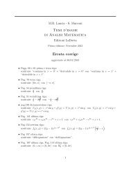
Here is the case of a service pole at the origin,with a residence pole at (L, H), with anetwork Σ. We take A(t) = t.HΣLThe optimal pricing policy B(t) is given byB(t) = (H 2 + L 2 ) 1/2 − (H 2 + (L − t) 2 ) 1/2 .1.210.80.60.40.20.5 1 1.5 2The case L = 2 and H = 1.34

Here is another case, with a single servicepole at the origin, with two residence polesat (L, H 1 ) and (L, H 2 ), with a network Σ.H 2ΣL H 1The optimal pricing policy B(t) is then{B2 (t) in [0, T ]B(t) =B 2 (T ) − B 1 (T ) + B 1 (t) in [T, L] .1.210.80.60.40.20.5 1 1.5 2The case L = 2, H 1 = 0.5, H 2 = 2.35

Problem 3 - Optimal City StructuresWe consider the following model for the optimalplanning of an urban area (Buttazzo-Santambrogio SIAM M.A. 2005).• Ω the geographical region or urban areaa compact regular domain of R N• f + the density of residentsa probability measure on Ω• f − the density of servicesa probability measure on Ω.Here the distance d in Ω is fixed (for simplicitywe take the Euclidean one) while theunknowns are f + and f − that have to bedetermined in an optimal way taking intoaccount the following facts:36

• there is a transportation cost for movingfrom the residential areas to the servicespoles;• people desire not to live in areas wherethe density of population is too high;• services need to be concentrated as muchas possible, in order to increase efficiencyand decrease management costs.The transportation cost will be describedthrough a Monge-Kantorovich mass transportationmodel; it is indeed given by a p-Wasserstein distance (p ≥ 1) W p (f + , f − ),being p = 1 the classical Monge case.The total unhappiness of citizens due tohigh density of population will be describedby a penalization functional, of the form{ ∫H(f + h(u) dx) = Ω if f + = u dx+∞ otherwise,37

where h is assumed convex and superlinear(i.e. h(t)/t → +∞ as t → +∞). The increasingand diverging function h(t)/t thenrepresents the unhappiness to live in an areawith population density t.Finally, there is a third term G(f − ) whichpenalizes sparse services. We force f − tobe a sum of Dirac masses and we considerG(f − ) a functional defined on measures,of the form studied by Bouchitté-Buttazzo(Nonlinear An. 1990, IHP 1992, IHP 1993):{ ∑G(f − ) = n g(a n) if f − = ∑ n a nδ xn+∞ otherwise,where g is concave and with infinite slopeat the origin. Every single term g(a n ) inthe sum represents here the cost for buildingand managing a service pole of dimensiona n , located at the point x n ∈ Ω.38

We have then the optimization problem{min W p (f + , f − ) + H(f + ) + G(f − ) :}f + , f − probabilities on Ω .Theorem There exists an optimal pair(f + , f − ) solving the problem above.Also in this case we obtain some necessaryconditions of optimality. In particular, ifΩ is sufficiently large, the optimal structureof the city consists of a finite number ofdisjoint subcities: circular residential areaswith a service pole at the center.39

Problem 4 - Optimal Riemannian MetricsHere the domain Ω and the probabilities f +and f − are given, whereas the distance dis supposed to be conformally flat, that isgenerated by a coefficient a(x) through theformula{ ∫ 1d a (x, y) = inf a ( γ(t) ) |γ ′ (t)| dt :0}γ ∈ Lip(]0, 1[; Ω), γ(0) = x, γ(1) = y.We can then consider the cost functionalF (a) = MK(f + , f − , d a ).The goal is to prevent as much as possiblethe transportation of f + onto f − by maximizingthe cost F (a) among the admissiblecoefficients a(x). Of course, increasing a(x)would increase the values of the distance d a40

and so the value of the cost F (a). The classof admissible controls is taken as{A = a(x) Borel measurable :∫}α ≤ a(x) ≤ β, a(x) dx ≤ m .In the case when f + = δ x and f − = δ yare Dirac masses concentrated on two fixedpoints x, y ∈ Ω, the problem of maximizingF (a) is nothing else than that of provingthe existence of a conformally flat Euclideanmetric whose geodesics joining x and y areas long as possible.This problem has several natural motivations;indeed, in many concrete examples,one can be interested in making as difficultas possible the communication betweenΩsome masses f + and f − .For instance, itis easy to imagine that this situation may41

arise in economics, or in medicine, or simplyin traffic planning, each time the connectionbetween two “enemies” is undesired.Of course, the problem is made non trivialby the integral constraint ∫ a(x) dx ≤ m,Ωwhich has a physical meaning: it prescribesthe quantity of material at one’s disposal tosolve the problem.The analogous problem of minimizing thecost functional F (a) over the class A, whichcorresponds to favor the transportation off + into f − , is trivial, sinceinf{}F (a) : a ∈ A= F (α).The existence of a solution for the maximizationproblemmax{}F (a) : a ∈ A42

is a delicate matter. Indeed, maximizingsequences {a n } ⊂ A could develop an oscillatorybehavior producing only a relaxedsolution. This phenomenon is well known;basically what happens is that the class A isnot closed with respect to the natural convergencea n → a ⇐⇒ d an → d a uniformlyand actually it can be proved that A is densein the class of all geodesic distances (in particular,in all the Riemannian ones).Nevertheless, we were able to prove the followingexistence result.Theorem The maximization problem aboveadmits a solution in a opt ∈ A.43

Several questions remain open:• Under which conditions is the optimal solutionunique?• Is the optimal solution of bang-bang type?In other words do we have a opt ∈ {α, β}or intermediate values (homogenization)are more performant?• Can we characterize explicitely the optimalcoefficient a opt in the case f + = δ x andf − = δ y ?44

Some Numerical ComputationsHere are some numerical computations performed(Buttazzo-Oudet-Stepanov 2002) inthe simpler case of the so-called problem ofoptimal irrigation.This is the optimal network Problem 1 inthe case f − ≡ 0, where customers only wantto minimize the averaged distance from thenetwork.In other words, the optimization criterionbecomes simply∫F (Σ) = dist(x, Σ) df + (x) .ΩDue to the presence of many local minimathe method is based on a genetic algorithm.45

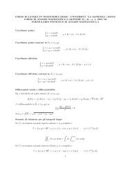
Optimal sets of length 0.5 and 1 in a unit diskOptimal sets of length 1.25 and 1.5 in a unit diskOptimal sets of length 2 and 3 in a unit disk46

Optimal sets of length 0.5 and 1 in a unit squareOptimal sets of length 1.5 and 2.5 in a unit squareOptimal sets of length 3 and 4 in a unit square47

Optimal sets of length 1 and 2 in the unit ball of R 3Optimal sets of length 3 and 4 in the unit ball of R 348

Now we give a model that takes into accountwhat occurs in several natural structures(see figures above). Indeed, they presentsome interesting features that should be interpretedin terms of mass transportation.However the usual Monge-Kantorovich theorydoes not provide an explaination to thereasons for which the structures above exist,and it cannot be taken as a mathematicalmodel for them. For instance, if the sourceis a Dirac mass and the target is a segment,as in figure below, the Monge-Kantorovichtheory provides a wrong behaviour.The Monge transport rays.49

Various approaches have been proposed togive more appropriated models:• Q. Xia (Comm. Cont. Math. 2003)through the minimization of a suitablefunctional defined on currents;• V. Caselles, J. M. Morel, S. Solimini, . . .(Preprint 2003 http://www.cmla.enscachan.fr/Cmla/,Interfaces and FreeBoundaries 2003, PNLDE 51 2002) througha kind of analogy of fluid flow in thintubes.• A. Brancolini, G. Buttazzo, E. Oudet, E.Stepanov, (see http://cvgmt.sns.it)through a variational model for irrigationtrees.Here we propose a different approach basedon a definition of path length in a Wassersteinspace.50

We also give a model where the oppositefeature occurs: instead of favouring the concentrationof transport rays, the variationalfunctional prevents it giving a lower cost todiffused measures.The mathematical model will be consideredin an abstract metric space frameworkwhere both behaviours (favouring concentrationand diffusion) are included; we donot know of natural phenomena where thediffusive behaviour occurs.The results presented here are contained inA. Brancolini, G. Buttazzo, F. Santambrogio:Path functionals over Wassersteinspaces. Preprint 2004, available athttp://cvgmt.sns.it51

We consider an abstract framework wherea metric space X with distance d is given.We assume that closed bounded subsets ofX are compact. Fix two points x 0 and x 1in X and consider the path functionalJ (γ) =∫ 10J(γ(t))|γ ′ |(t) dtwhere γ : [0, 1] → X ranges among allLipschitz curves such that γ(0) = x 0 andγ(1) = x 1 . Here:• J : X → [0, +∞] is a given mapping onX;• |γ ′ |(t) is the metric derivative of γ at thepoint t, i.e.|γ ′ |(t) = lim sups→td ( γ(s), γ(t) )|s − t|.52

Theorem Assume:• J is lower semicontinuous in X;• J ≥ c with c > 0, or more generally∫ +∞ (infB(r) J ) dr = +∞.0Then, for every x 0 , x 1 ∈ X there exists anoptimal path for the problem}min{J (γ) : γ(0) = x 0 , γ(1) = x 1provided there exists a curve γ 0 , connectingx 0 to x 1 , such that J (γ 0 ) < +∞.The application of the theorem above consistsin taking as X a Wasserstein spaceW p (Ω) where Ω is a compact metric spaceequipped with a distance function c anda positive finite non-atomic Borel measurem (usually a compact of R N with the Euclideandistance and the Lebesgue measure).53

We recall that, in the case Ω compact,W p (Ω) is the space of all Borel probabilitymeasures µ on Ω equipped with the p-Wasserstein distance( ∫w p (µ 1 , µ 2 ) = infΩ×Ω) 1/pc(x, y) p λ(dx, dy)where the infimum is taken on all transportplans λ between µ 1 and µ 2 , that is onall probability measures λ on Ω × Ω whosemarginals π # 1 λ and π# 2 λ coincide with µ 1and µ 2 respectively.In order to define the functionalJ (γ) =∫ 10J(γ(t))|γ ′ |(t) dtit remains to fix the “coefficient” J.Wetake a l.s.c. functional on the space of measures,of the kind considered by Bouchittéand Buttazzo (Nonlinear Anal. 1990, Ann.IHP 1992, Ann. IHP 1993):54

∫∫ ∫J(µ) = f(µ a )dm+ f ∞ (µ c )+ g(µ(x))d#ΩΩΩwhere• µ = µ a · m + µ c + µ # is the Lebesgue-Nikodym decomposition of µ with respectto m, into absolutely continuous,Cantor, and atomic parts;• f : R → [0, +∞] is convex, l.s.c.proper;• f ∞ is the recession function of f;and• g : R → [0, +∞] is l.s.c. and subadditive,with g(0) = 0;• # is the counting measure;• f and g verify the compatibility conditionlimt→+∞f(ts)t= limt→0 + g(ts)t.55

In this way the functional J is l.s.c. for theweak* convergence of measures. If we furtherassume that f(s) > 0 for s > 0 andg(1) > 0, then we have J ≥ c > 0. The existencetheorem then applies and, given twoprobabilities µ 0 and µ 1 , we obtain at leasta minimizing path for the problem}min{J (γ) : γ(0) = µ 0 , γ(1) = µ 1 .provided J is not identically +∞.We now study two special cases (Ω ⊂ R Ncompact and m = dx):Concentration f ≡ +∞, g(z) = |z| rr ∈]0, 1[. We have then∫J(µ) = |µ(x)| r d#Ωµ atomicwithDiffusion f(z) = |z| q with q > 1, g ≡ +∞.We have then∫J(µ) = |u(x)| q dx µ = u · dx, u ∈ L q .Ω56

Concentration case. The following factsin the concentration case hold:• If µ 0 and µ 1 are convex combinations(also countable) of Dirac masses, thenthey can be connected by a path γ(t) offinite minimal cost J .• If r > 1 − 1/N then every pair of probabilitiesµ 0 and µ 1 can be connected by apath γ(t) of finite minimal cost J .• The bound above is sharp. Indeed, if r ≤1 − 1/N there are measures that cannotbe connected by a finite cost path (forinstance a Dirac mass and the Lebesguemeasure).57

Example. (Y-shape versus V-shape). Wewant to connect (concentration case r < 1fixed) a Dirac mass to two Dirac masses (ofweight 1/2 each) as in figure below, l and hare fixed. The value of the functional J isgiven byJ (γ) = x + 2 1−r√ (l − x) 2 + h 2 .Then the minimum is achieved forhx = l − √41−r− 1 .When r = 1/2 we have a Y-shape if l > hand a V-shape if l ≤ h.•h•xl•A Y-shaped path for r = 1/2.58

Diffusion case. The following facts in thediffusion case hold:• If µ 0 and µ 1 are in L q (Ω), then they canbe connected by a path γ(t) of finite minimalcost J . The proof uses the displacementconvexity (McCann 1997) which,for a functional F and every µ 0 , µ 1 , is theconvexity of the map t ↦→ F (T (t)), beingT (t) = [(1 − t)Id + tT ] # µ 0 and T an optimaltransportation between µ 0 and µ 1 .• If q < 1 + 1/N then every pair of probabilitiesµ 0 and µ 1 can be connected by apath γ(t) of finite minimal cost J .• The bound above is sharp. Indeed, if q ≥1 + 1/N there are measures that cannotbe connected by a finite cost path (forinstance a Dirac mass and the Lebesguemeasure).59

The previous existence results were basedon two important assumptions:• the compactness of Wasserstein spacesW p (Ω) for Ω compact and 1 ≤ p < +∞;• the estimate like F q ≥ c > 0, that can beobtained when |Ω| < +∞.Both the facts do not hold when Ω is unbounded(indeed, the corresponding Wassersteinspaces are not even locally compact).The same happens when Ω is compact butwe consider the space W ∞ (Ω).Here is a more refined abstract setting whichadapts to the unbounded case.Notice that in the unbounded case theWasserstein spaces W p (Ω) do not contain allthe probabilities on Ω but only those withfinite momentum of order p., that is∫|x| p µ < +∞ .Ω60

Theorem Let (X, d, d ′ ) be a metric spacewith two different distances. Assume that:• d ′ ≤ d;• all d-bounded sets in X are relativelycompact with respect to d ′ ;• the mapping d : X × X → R + is a lowersemicontinuous function with respect tothe distance d ′ × d ′ .Consider a functional J : X → [0, +∞] andassume that:• J is d ′ -l.s.c.;• ∫ +∞ (infBd0(r) J ) dr = +∞.Then the functionalJ (γ) =∫ 10J(γ(t))|γ ′ | d (t) dthas a minimizer on the set of d−Lipschitzcurves connecting two given points x 0 andx 1 , provided it is not identically +∞.61

As an application of the theorem above weconsider the diffusion case when Ω = R N .The concentration case in the unboundedsetting still presents some extra difficultiesthat we did not yet solve. We take:• d the Wasserstein distance;• d ′ the distance metrizing the weak* topologyon probabilities:d ′ (µ, ν) =∞∑k=12 −k1 + c k∣ ∣〈φk , µ − ν〉 ∣ ∣where (φ k ) is a dense sequence of Lipschitzfunctions in the unit ball of C b (Ω)and c k are their Lipschitz constants.We may prove that the assumptions of theabstract scheme are fulfilled, and we have(for the diffusion case):62

• if q < 1 + 1/N for every µ 0 and µ 1 thereexists a path giving finite and minimalvalue to the cost J ;• if q ≥ 1 + 1/N there exist measures µ 0(actually a Dirac mass) such that J =+∞ on every nonconstant path startingfrom µ 0 .Open Problems• linking two L q measures in the diffusionunboundedcase;• concentration case in unbounded setting;• Ω unbounded but not necessarily thewhole space;• working with the space W ∞ (Ω);• comparing this model to the ones by Xiaand by Morel, Solimini, . . . ;• numerical computations;• evolution models?63

References(all available at http://cvgmt.sns.it)A. Brancolini, G. Buttazzo: Optimalnetworks for mass transportation problems.Esaim COCV (to appear).G. Buttazzo, A. Davini, I. Fragalà,F. Macià: Optimal Riemannian distancespreventing mass transfer. J. Reine Angew.Math., (to appear).G. Buttazzo, E. Oudet, E. Stepanov:Optimal transportation problems with freeDirichlet regions. In PNLDE 51, BirkhäuserVerlag, Basel (2002), 41–65.G. Buttazzo, A. Pratelli, E. Stepanov:Optimal pricing policies for public transportationnetworks. Preprint Dipartimentodi Matematica Università di Pisa, Pisa (2004).G. Buttazzo, F. Santambrogio: A Modelfor the Optimal Planning of an Urban Area.Preprint Dipartimento di Matematica Universitàdi Pisa, Pisa (2003).64