Maple Solutions to the Chemical Engineering Problem Set
Maple Solutions to the Chemical Engineering Problem Set
Maple Solutions to the Chemical Engineering Problem Set

Create successful ePaper yourself
Turn your PDF publications into a flip-book with our unique Google optimized e-Paper software.
⎡ 0<br />
⎢ 9<br />
⎢<br />
⎢10<br />
⎢<br />
⎢11<br />
⎢<br />
⎢12<br />
⎢<br />
⎢13<br />
⎢<br />
⎢14<br />
⎢<br />
⎢15<br />
⎢<br />
⎢16<br />
⎢<br />
⎢17<br />
⎢<br />
⎢18<br />
⎢<br />
⎢19<br />
⎢<br />
⎣20<br />
80<br />
80<br />
80.00000516<br />
77.64681396<br />
75.58158780<br />
73.82512871<br />
72.40877288<br />
71.36231380<br />
70.70902677<br />
70.46248083<br />
70.62437518<br />
71.18325249<br />
72.11402574<br />
80<br />
80<br />
79.99999484<br />
79.64269439<br />
77.59747344<br />
75.57269420<br />
73.82166335<br />
72.40641866<br />
71.36074478<br />
70.70837739<br />
70.46288279<br />
70.62589984<br />
71.18590699<br />
80<br />
80<br />
80.<br />
80.02650031<br />
79.76982224<br />
79.18312375<br />
78.35992679<br />
77.39937837<br />
76.39059205<br />
75.41166771<br />
74.52992468<br />
73.80184548<br />
73.27275148<br />
0 ⎤<br />
⎥<br />
0 ⎥<br />
0 ⎥<br />
-.02217814937 ⎥<br />
.04954268262 ⎥<br />
.5490806715 ⎥<br />
1.762104706 ⎥<br />
3.874889469 ⎥<br />
6.979304493 ⎥<br />
11.08363213 ⎥<br />
16.12345525 ⎥<br />
21.97243756 ⎥<br />
28.45330713 ⎦<br />
The first column is <strong>the</strong> time, <strong>the</strong> next three are <strong>the</strong> tank, <strong>the</strong>rmocouple, and measured temperatures.<br />
A. Open Loop Performance<br />
Open loop performance is simulated by setting K = 0, which is what was done for <strong>the</strong> above<br />
c<br />
calculations. We need <strong>to</strong> integrate for a longer time, however, so we repeat <strong>the</strong> above command but<br />
integrate <strong>to</strong> 60 minutes.<br />
> result:=dsolve({diff(x(t),t)=0,diff(y(t),t)=0,diff(w(t),t)=0,diff(z(t),t)=0}, {w(t),x(t),y(t),z(t)},type=numeric,<br />
method=rkf45, initial=vec<strong>to</strong>r([80,80,80,0]),start=0,procedure=deproc,value=array([0,seq(i,i=9..60)]));<br />
We extract <strong>the</strong> results table<br />
> Ttable :=op([1,3,2,2],result):<br />
and plot <strong>the</strong> three temperatures.<br />
> with(linalg):<br />
> plot({seq([seq([Ttable[i,1],Ttable[i,k]],i=1..rowdim(Ttable))],k=2..4)},color=[red,blue,black]);<br />
80<br />
75<br />
70<br />
65<br />
60<br />
0<br />
10<br />
20<br />
30<br />
40<br />
50<br />
60<br />
B. Closed loop performance<br />
This requires a change in K c <strong>to</strong> 50 (it was 0 in <strong>the</strong> first case).<br />
> params :={V=4000/rho/C[P],W=500/C[P],T[i,s]=60,T[r]=80,tau[d]=1,tau[m]=5,tau[I]=2,K[c]=50};<br />
Page 46