Maple Solutions to the Chemical Engineering Problem Set

100
95
90
85
80
75
70
65
0
50
100
150
200
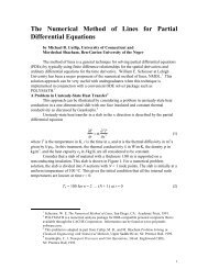
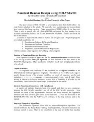
D. Proportional Control
K
c
Proportional only control is simulated by setting the term = 0. We can accomplish this by giving τ a
τ I
I
very high value as shown here.
> params :={V=4000/rho/C[P],W=500/C[P],T[i,s]=60,T[r]=80,tau[d]=1,tau[m]=5,tau[I]=1e99,K[c]=500};
4000
params := { V = , W = , , , , , ,
}
ρC
P
500
T = 60 T = 80 τ = 1 τ = 5 τ = .1 10
C i, s r d m I
P
100
K = 500
c
We carry out the integrations for this situation.
> result:=dsolve({diff(x(t),t)=0,diff(y(t),t)=0,diff(w(t),t)=0,diff(z(t),t)=0}, {w(t),x(t),y(t),z(t)},type=numeric,
method=rkf45, initial=vector([80,80,80,0]),start=0,procedure=deproc,
value=array([0,seq(i,i=9..60)])):
The output table is extracted from the result:
> Ttable :=op([1,3,2,2],result):
and the three temperatures plotted as a function of time.
> plot({seq([seq([Ttable[i,1],Ttable[i,k]],i=1..rowdim(Ttable))],k=2..4)},color=[red,blue,black]);
>
80
78
76
74
72
70
0
10
20
30
40
50
60
Page 48