Fluid mechanics of fibre suspensions related to papermaking - DiVA

∂W
∂t
+ U ∂W
∂x
− ∂P
∂z
+ ν
2.1. TWO-PHASE FLOW 11
∂W ∂W
+ V + W
∂y ∂z =
2 ∂ W
∂x2 + ∂2W ∂y2 + ∂2W ∂z2
∂uw ∂vw ∂w2
− + + . (2.12)
∂x ∂y ∂z
The continuity equation becomes
∂U
∂x
+ ∂U
∂y
+ ∂U
∂z
= 0, (2.13)
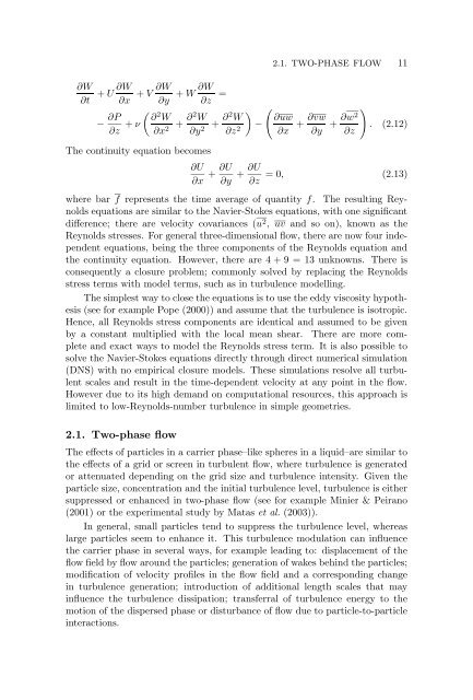
where bar f represents the time average of quantity f. The resulting Reynolds
equations are similar to the Navier-Stokes equations, with one significant
difference; there are velocity covariances (u 2 , uv and so on), known as the
Reynolds stresses. For general three-dimensional flow, there are now four independent
equations, being the three components of the Reynolds equation and
the continuity equation. However, there are 4 + 9 = 13 unknowns. There is
consequently a closure problem; commonly solved by replacing the Reynolds
stress terms with model terms, such as in turbulence modelling.
The simplest way to close the equations is to use the eddy viscosity hypothesis
(see for example Pope (2000)) and assume that the turbulence is isotropic.
Hence, all Reynolds stress components are identical and assumed to be given
by a constant multiplied with the local mean shear. There are more complete
and exact ways to model the Reynolds stress term. It is also possible to
solve the Navier-Stokes equations directly through direct numerical simulation
(DNS) with no empirical closure models. These simulations resolve all turbulent
scales and result in the time-dependent velocity at any point in the flow.
However due to its high demand on computational resources, this approach is
limited to low-Reynolds-number turbulence in simple geometries.
2.1. Two-phase flow
The effects of particles in a carrier phase–like spheres in a liquid–are similar to
the effects of a grid or screen in turbulent flow, where turbulence is generated
or attenuated depending on the grid size and turbulence intensity. Given the
particle size, concentration and the initial turbulence level, turbulence is either
suppressed or enhanced in two-phase flow (see for example Minier & Peirano
(2001) or the experimental study by Matas et al. (2003)).
In general, small particles tend to suppress the turbulence level, whereas
large particles seem to enhance it. This turbulence modulation can influence
the carrier phase in several ways, for example leading to: displacement of the
flow field by flow around the particles; generation of wakes behind the particles;
modification of velocity profiles in the flow field and a corresponding change
in turbulence generation; introduction of additional length scales that may
influence the turbulence dissipation; transferral of turbulence energy to the
motion of the dispersed phase or disturbance of flow due to particle-to-particle
interactions.