REPLACEMENT SENSOR MODEL (RSM) PERFORMANCE ... - asprs

More documents

Recommendations

Info

covariance mapping (see the following section). These times are for a single Pentium processor running at 1.86 GHz. No effort has been made to optimize the time performance of the RSM Generator, which tends to be limited by the time for the original sensor model projective model calls for the fitting and evaluation points. In addition to the ground-to-image calls needed to populate the interpolating grid, the 110 coefficients of the baseline polynomial (55 for row and 55 for column) are calculated by calling the original sensor model image-to-ground function at 1000 fitting points, and the original sensor model image-to-ground function is also called at the 1000 randomly generated evaluation points. The polynomial for the baseline projective model is in a single section covering the entire image. The RSM Generator automatically divides the interpolating grid into sections as needed in order to be represented within the RSMSD format. For QuickBird a single section was used, and for WorldView about 32 sections were used for each image. 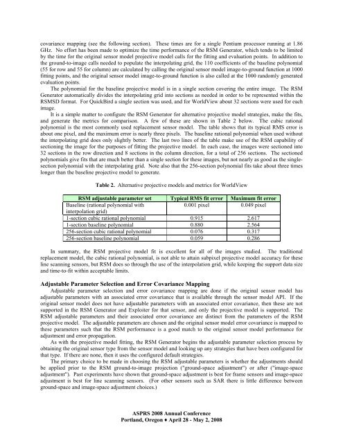It is a simple matter to configure the RSM Generator for alternative projective model strategies, make the fits, and generate the metrics for comparison. A few of these are shown in Table 2 below. The cubic rational polynomial is the most commonly used replacement sensor model. The table shows that its typical RMS error is about one pixel, and the maximum error is nearly three pixels. The baseline rational polynomial when used without the interpolating grid does only slightly better. The last two lines of the table make use of the RSM capability of sectioning the image for the purposes of fitting the projective model. In each case, the images were sectioned into 32 sections in the row direction and 8 sections in the column direction, for a total of 256 sections. The sectioned polynomials give fits that are much better than a single section for these images, but not nearly as good as the singlesection polynomial with the interpolating grid. Note also that the 256-section polynomial fits take about three times longer than the baseline projective model to generate. Table 2. Alternative projective models and metrics for WorldView RSM adjustable parameter set Typical RMS fit error Maximum fit error Baseline (rational polynomial with interpolation grid) 0.001 pixel 0.049 pixel 1-section cubic rational polynomial 0.915 2.617 1-section baseline polynomial 0.880 2.564 256-section cubic rational polynomial 0.076 0.317 256-section baseline polynomial 0.059 0.286 In summary, the RSM projective model fit is excellent for all of the images studied. The traditional replacement model, the cubic rational polynomial, is not able to attain subpixel projective model accuracy for these line scanning sensors, but RSM does so through the use of the interpolation grid, while keeping the support data size and time-to-fit within acceptable limits. Adjustable Parameter Selection and Error Covariance Mapping Adjustable parameter selection and error covariance mapping are done if the original sensor model has adjustable parameters with an associated error covariance that is available through the sensor model API. If the original sensor model does not have adjustable parameters with an associated error covariance, then these are not supported in the RSM Generator and Exploiter for that sensor, and only the projective model is supported. The RSM adjustable parameters and their associated error covariance are distinct from the parameters of the RSM projective model. The adjustable parameters are chosen and the original sensor model error covariance is mapped to these parameters such that the RSM performance is a good match to the original sensor model performance for adjustment and error propagation. As with the projective model fitting, the RSM Generator begins the adjustable parameter selection process by obtaining the original sensor type from the sensor model and looking up any strategies that have been configured for that type. If there are none, then it uses the configured default strategies. The primary choice to be made in choosing the RSM adjustable parameters is whether the adjustments should be applied prior to the RSM ground-to-image projection ("ground-space adjustment") or after ("image-space adjustment"). Past experiments have shown that ground-space adjustment is best for frame sensors and image-space adjustment is best for line scanning sensors. (For other sensors such as SAR there is little difference between ground-space and image-space adjustment choices.) ASPRS 2008 Annual Conference Portland, Oregon ♦ April 28 - May 2, 2008
Another choice to be made is which specific ground- or image-space adjustment parameters are to be considered, and whether the best linear combinations of the parameters are to be used or whether the parameters are to be used without being combined. The former is recommended by the RSM development team, and it requires the updated RSMSD format. When the choice is made to use the best linear combinations of the RSM adjustable parameters, the RSM Generator performs a principal components analysis of the RSM adjustable parameter error covariance, and selects enough of the resulting eigenvectors to match the original sensor model performance faithfully. The error covariance condition number is also computed and used as a criterion in the selection process. (The condition number computation insures that the RSM adjustable error covariance is a legitimate positive-definite matrix and gives confidence that the adjustment and error propagations that use it will be numerically stable.) Since the RSM adjustable parameter error covariance is diagonal when expressed in terms of the principal components, it results in very stable performance in adjustment. Note that the "choices" above are made when the RSM Generator is configured. In normal operation, the adjustable parameter selection and covariance mapping (and indeed all of the steps of the RSMSD generation) are done automatically by the RSM Generator, with no operator interaction required. The error covariance mapping is done as described in the Manual of Photogrammetry article referenced in the introduction. This process requires the original sensor model, from which the RSM Generator obtains the adjustable parameters and their error covariance. The a priori QuickBird adjustable parameter error covariance used was the default covariance coded in Socet Set. Since the Socet Set WorldView sensor model was coded prior to the calibration of the WorldView sensor, the coded defaults were not used. An a priori error covariance consistent with the WorldView specification was used instead. A few quick experiments with QuickBird and WorldView confirmed our earlier findings that image-space adjustable parameters perform well for line-scanning sensors. The image-space adjustable parameters are two correction polynomials, one for image row (line) and one for image column (sample), that are applied after the projective model computations in the ground-to-image function as explained in the companion paper. We chose to allow linear combinations of image space corrections as a function of the image-aligned rectangular coordinates, with terms up to third order in X and Y and up to first order in Z, with cross-terms up to a maximum combined order of 3. This is a total of 32 terms, from which the RSM Generator chooses the best linear combinations. Since the number of original sensor model adjustable parameters is 6, the number of combinations must also be 6 or less, and 6 were used. The adjustable parameter selection and covariance mapping metrics are summarized in Table 3. The normalized frobenius norm of the residual adjustable parameter error covariance projected to image space is a covariance mapping metric that can be regarded as a fractional error in the process. The maximum for either image type is much less than 0.01, and the smaller the normalized frobenius norm the better the covariance mapping. The condition numbers of the error covariances are shown as well. The smaller the condition number the more stable the error covariance is likely to be in adjustment and error propagation computations. Table 3. Adjustable parameter selection and error covariance mapping statistics for QuickBird and WorldView RSM projective model fitting statistic QuickBird WorldView Typical normalized frobenius norm 0.0016 0.000783 Maximum normalized frobenius norm 0.0039 0.000836 Typical condition number 3.5e+4 4.0e+6 Maximum condition number 1.11e+6 1.14e+7 It is instructive to compare the metrics of the adjustable parameter selection and error covariance mapping process with those of other potential RSM adjustable parameter sets. This comparison can be seen in Table 4 for the WorldView test images and three variations on the adjustable parameter set. With six ground-space adjustable parameters, a set that typically works well for frame images, the normalized frobenius norm is about three times larger than for the baseline set, which is still good, but the condition number is up to two orders of magnitude larger, so that solutions are not as stable. The 6-parameter image-space adjustment that is linear in image coordinates is a set sometimes used with RPC replacement models, despite the fact that the NITF TREs aren't capable of transmitting the error covariance. Its normalized frobenius norm is about four times larger than for the baseline set and the condition number is up to an order of magnitude larger. The 2-parameter image space offsets have a much lower fidelity with a normalized frobenius norm over ten times larger than for the baseline set. The condition number is of course much smaller than for the baseline case since there are only two parameters. ASPRS 2008 Annual Conference Portland, Oregon ♦ April 28 - May 2, 2008
Page 1 and 2: REPLACEMENT SENSOR MODEL (RSM) PERF
Page 3: For the commercial satellite study
Page 7 and 8: and for the stereo pair. The origin
Page 9 and 10: In the two test procedures already
Page 11: good fit to the original, but the e

REPLACEMENT SENSOR MODEL (RSM) PERFORMANCE ... - asprs

Create successful ePaper yourself

Delete template?

Save as template?