Consistent chiral three-nucleon interactions in ... - Theory Center

4 Three-body Jacobi matrix element transformation into the m-scheme
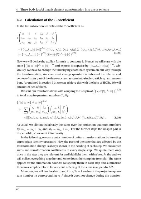
4.2 Calculation of the T -coefficient
In the last subsection we defined the T-coefficient as
⎛
⎞
a b c Jab J J
⎜
⎟
T⎝
⎠
ncm lcm n12 l12 n3 l3
sab j12 j3 tab T MT
= 〈ncmlcm| ⊗ 〈α| J M
|{[(nala, sa)ja, (nblb, sb)jb]Jab, (nclc, sc)jc}J M, tamtatbmtb tcmtc〉
:= 〈ncmlcm| ⊗ 〈α| J M
Jab
J M (4.28)
{|a〉 ⊗ |b〉} ⊗ |c〉 .
Now we will derive the explicit formula to compute it. Hence, we will start with the
state {|a〉 ⊗ |b〉} Jab ⊗ |c〉 J M and express it stepwise by |ncmlcm〉 ⊗ |α〉 J M . Ob-
viously, we have to change the underlying coordinate system on our way through
the transformation, since we must change quantum numbers of the relative and
center-of-mass part of the three-nucleon system into single-particle quantum num-
bers. As outlined in section 3.3, we can achieve this with the help of HOBs. We will
encounter two of them.
We start our transformations with coupling the isospin of {|a〉⊗|b〉} Jab⊗|c〉 J M
to total isospin quantum numbers T, MT
Jab
J M
{|a〉 ⊗ |b〉} ⊗ |c〉
=
ta tb tab
tab,T
mta mtb
mtab
tab tc
mtab tc
T
MT
×|{[(nala, sa)ja, (nblb, sb)jb]Jab, (nclc, sc)jc}J M, [(ta, tb)tab, tc]TMT 〉 . (4.29)
As usual, we eliminated already the sums over the projection quantum numbers
by mtab = mta + mtb and MT = mtab + mtc. For the further steps the isospin part is
dispensable, so we omit it for brevity.
In the following, we carry out a number of unitary transformations by inserting
appropriate identity operators. How the parts of the state that are affected by the
transformation change is always shown in the heading of each step. We encounter
sums and transformation coefficients in every single step. We quote them only
once in the step they are relevant for and highlight them with a box. At the end we
will collect everything together and write down the complete formula. The same
applies for the summation bounds: we specify them in each step and summarize
them in a simplified form for a special ordering of the sums in appendix A.2.
Moreover, we will use the shorthand ˆx = √ 2x + 1 and omit the projection quan-
tum number M corresponding to J since it does not change during the transfor-
46