LR Rabiner and RW Schafer, June 3

DRAFT: L. R. Rabiner and R. W. Schafer, June 3, 2009
8.2. HOMOMORPHIC SYSTEMS FOR CONVOLUTION 435
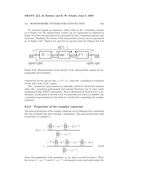
To represent signals as sequences, rather than in the z-transform domain
as in Figure 8.8, the characteristic system can be represented as depicted in
Figure 8.9 where the log function is surrounded by the z-transform operator and
its inverse. Similarly, the inverse of the characteristic system can be represented
as in Figure 8.10. Figures 8.5 and 8.6 are special cases for Figures 8.9 8.10
−1
D∗
{ }
+ + + • • *
Z { } exp{
} -1
yn ˆ[ ]
Yˆ Z { }
( z)
Y( z)
yn [ ]
yˆ 1[
n]
∗ yˆ
2[
n]
y1[ n]
∗ y2[
n]
Figure 8.10: Representation of the inverse of the characteristic system for homomorphic
deconvolution.
respectively for the special case z = e jω , i.e., when the z-transform is evaluated
on the unit circle of the z-plane.
The z-transform representation is especially useful for theoretical analysis
where the z-transform polynomials and rational functions can be more easily
manipulated than DTFT expressions. This is illustrated in Section 8.2.3. Furthermore,
as discussed in Section 8.4.2, if a powerful root solver is available, the
z-transform representation is the basis of a method for computing the complex
cepstrum.
8.2.3 Properties of the complex cepstrum
The general properties of the complex cepstrum can be illustrated by considering
the case of signals that have rational z-transforms. The most general form that
is necessary to consider is
X(z) =
=
Mi
A
k=1
(1 − akz −1 Mo
)
(1 − b −1
k=1
Ni
(1 − ckz −1 )
k=1
k=1
k=1
k z−1 )
z −Mo Mo
A (−b −1
k )
Mi
(1 − akz −1 Mo
) (1 − bkz)
Ni
(1 − ckz −1 )
k=1
k=1
(8.19)
where the magnitudes of the quantities, ak, bk, and ck are all less than 1. Thus,
the terms (1 − akz −1 ) and (1 − ckz −1 ) correspond to zeros and poles inside the