LR Rabiner and RW Schafer, June 3
LR Rabiner and RW Schafer, June 3
LR Rabiner and RW Schafer, June 3

You also want an ePaper? Increase the reach of your titles
YUMPU automatically turns print PDFs into web optimized ePapers that Google loves.
DRAFT: L. R. <strong>Rabiner</strong> <strong>and</strong> R. W. <strong>Schafer</strong>, <strong>June</strong> 3, 2009<br />
470CHAPTER 8. THE CEPSTRUM AND HOMOMORPHIC SPEECH PROCESSING<br />
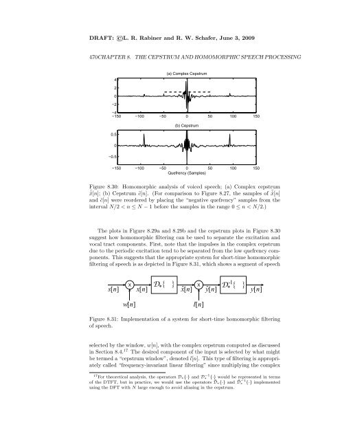
4<br />
2<br />
0<br />
−2<br />
(a) Complex Cepstrum<br />
−4<br />
−150 −100 −50 0 50 100 150<br />
0.5<br />
0<br />
−0.5<br />
(b) Cepstrum<br />
−150 −100 −50 0<br />
Quefrency (Samples)<br />
50 100 150<br />
Figure 8.30: Homomorphic analysis of voiced speech; (a) Complex cepstrum<br />
˜ˆx[n]; (b) Cepstrum ˜c[n]. (For comparison to Figure 8.27, the samples of ˜ ˆx[n]<br />
<strong>and</strong> ˜c[n] were reordered by placing the “negative quefrency” samples from the<br />
interval N/2 < n ≤ N − 1 before the samples in the range 0 ≤ n < N/2.)<br />
The plots in Figure 8.29a <strong>and</strong> 8.29b <strong>and</strong> the cepstrum plots in Figure 8.30<br />
suggest how homomorphic filtering can be used to separate the excitation <strong>and</strong><br />
vocal tract components. First, note that the impulses in the complex cepstrum<br />
due to the periodic excitation tend to be separated from the low quefrency components.<br />
This suggests that the appropriate system for short-time homomorphic<br />
filtering of speech is as depicted in Figure 8.31, which shows a segment of speech<br />
s[ n]<br />
X X<br />
wn [ ]<br />
D { }<br />
-1{<br />
}<br />
∗<br />
xn [ ] xn ˆ[ ]<br />
ln [ ]<br />
D<br />
yn ˆ[ ] ∗ yn [ ]<br />
Figure 8.31: Implementation of a system for short-time homomorphic filtering<br />
of speech.<br />
selected by the window, w[n], with the complex cepstrum computed as discussed<br />
in Section 8.4. 17 The desired component of the input is selected by what might<br />
be termed a “cepstrum window”, denoted l[n]. This type of filtering is appropriately<br />
called “frequency-invariant linear filtering” since multiplying the complex<br />
17 −1<br />
For theoretical analysis, the operators D∗{·} <strong>and</strong> D∗ {·} would be represented in terms<br />
of the DTFT, but in practice, we would use the operators ˜ D∗{·} <strong>and</strong> ˜ D −1<br />
∗ {·} implemented<br />
using the DFT with N large enough to avoid aliasing in the cepstrum.