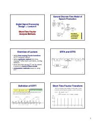
LR Rabiner and RW Schafer, June 3

More documents

Recommendations

Info

DRAFT: L. R. Rabiner and R. W. Schafer, June 3, 2009 474CHAPTER 8. THE CEPSTRUM AND HOMOMORPHIC SPEECH PROCESSING If, on the other hand, we do not know whether or not the input signal has the minimum-phase property, we can nevertheless assume that it does. Then the sequence ˆy[n] = lmnp[n]c[n] would be the complex cepstrum of a signal y[n] whose Fourier transform would have the same log magnitude as the Fourier transform of the original signal x[n]. If the original signal were not minimum-phase, arg{X(ejω )} and arg{Y (ejω )} would differ, but log |Y (ejω )| = log |X(ejω )|. If we assume that the low quefrencies in the cepstrum are due to the vocal tract system, and we further assume that the vocal tract system is minimum phase, then we can accomplish the estimation of a minimum-phase vocal tract impulse response by combining Eqs. (8.99a) and (8.96) to obtain ⎧ 0 n < 0 ⎪⎨ 1 n = 0 lmnp[n] = 2 0 < n < nco (8.99b) 1 n = nco ⎪⎩ 0 nco < n, which imposes a cutoff quefrency to remove the excitation components in the cepstrum and simultaneously imposes the minimum-phase condition. 19 Note that we have again included a one sample transition, which can be expanded if desired. For the voiced example of this section, the result of liftering the cepstrum in Figure 8.30b with the lowpass lifter in Eq. (8.99b) with cutoff quefrency nco = 50 is the impulse response shown in Figure 8.34b. From the above discussion, it follows that the log magnitude of the Fourier transform of the vocal tract impulse response estimate in Figure 8.34b is identical to that of the vocal tract impulse response estimate in Figure 8.32a since both were obtained with a cutoff quefrency of nco = 50; i.e., the smoothed log magnitude in Figure 8.29a is the log magnitude of the Fourier transform of both the waveforms in Figures 8.34b and 8.32a. In fact, the other two impulse response estimates in Figure 8.34a and 8.34c also have the same log magnitude of their Fourier transforms. The impulse response in Figure 8.34a corresponds to applying the lifter in Eq. (8.97) to the cepstrum (i.e., without incorporating the minimum-phase condition). This is equivalent to assuming that the phase is zero. The resulting impulse response is an even time sequence and is therefore non-causal. It could be made causal by truncating it symmetrically and introducing sufficient delay. The impulse response in Figure 8.34c is a maximum-phase impulse response that is obtained at the output after multiplying the cepstrum by lmxp[n] = lmnp[−n]; i.e., by imposing the maximum-phase condition that the complex cepstrum is zero for n > 0. The waveform of Figure 8.34c is seen to be a time-reversed version of the minimum-phase impulse response in Figure 8.34b. Again it can be made causal by truncating it and including sufficient delay. The effects of phase on synthetic speech reconstructed from impulse responses derived by homomorphic filtering were studied by Oppenheim [14] using vocal tract impulse responses derived by homomorphic filtering. The use of the cepstrum in speech coding is discussed in more detail in Chapter 11. 19 Observe that Eq. (8.99b) reduces to Eq. (8.99a) when nco → ∞.
DRAFT: L. R. Rabiner and R. W. Schafer, June 3, 2009 8.5. HOMOMORPHIC FILTERING OF NATURAL SPEECH 475 Amplitude 0.8 0.6 0.4 0.2 0 −0.2 (a) Zero−Phase Impulse Response Estimate −200 −150 −100 −50 0 50 100 150 200 0.4 0.2 0 −0.2 −0.4 (b) Minimum−Phase Impulse Response Estimate −200 −150 −100 −50 0 50 100 150 200 0.4 0.2 0 −0.2 −0.4 (c) Maximum−Phase Impulse Response Estimate −200 −150 −100 −50 0 Time (Samples) 50 100 150 200 Figure 8.34: Homomorphic filtering of voiced speech; (a) Zero-phase estimate of hV [n]; (b) Minimum-phase estimate of hV [n]; (c) Maximum-phase estimate of hV [n];. 8.5.5 Unvoiced Speech Analysis using the DFT To complete the illustration of homomorphic analysis of natural speech, consider the example of unvoiced speech given in Figure 8.35. Figure 8.35a shows a waveform segment of the fricative /SH/ multiplied by a 401-point Hamming window. The rapidly varying curve plotted with the thin line in Figure 8.35b is the corresponding log magnitude function log |X(e jω )|. Figure 8.35c shows the corresponding cepstrum c[n]. For consistency, and since we generally do not know in advance whether a particular speech segment is voiced or unvoiced, c[n] for unvoiced speech is computed as the inverse Fourier transform of log |X(e jω )| just as for voiced speech. Note the erratic variation of the log magnitude function (log periodogram). It is clear from Figure 8.35c that, in contrast to the case of voiced speech, the cepstrum of an unvoiced speech segment does not display any sharp peaks in the high quefrency region. Instead, the high quefrencies represent the rapid random fluctuations in Figure 8.35b. However, the low-time portion of the cepstrum can still be assumed to represent log |HU (e jω )|. This is illustrated in Figure 8.35b by the smooth curve plotted with the thick line, which represents the smoothed log magnitude function obtained by applying the lowpass cepstrum window of Eq. (8.96) to the cepstrum of Figure 8.35c with
Page 1 and 2: DRAFT: L. R. Rabiner and R. W. Scha
Page 51: DRAFT: L. R. Rabiner and R. W. Scha
Page 77: DRAFT: L. R. Rabiner and R. W. Scha

LR Rabiner and RW Schafer, June 3

You also want an ePaper? Increase the reach of your titles

Delete template?

Save as template?