- Page 2:
Fundamental Astronomy
- Page 5 and 6:
Dr. Hannu Karttunen University of T
- Page 7 and 8:
VI Preface to the First Edition The
- Page 9 and 10:
VIII Contents 5.6 Continuous Spectr
- Page 11 and 12:
X Contents 16. Star Clusters and As
- Page 14 and 15:
1. Introduction 1.1 TheRoleofAstron
- Page 16 and 17:
1.2 Astronomical Objects of Researc
- Page 18 and 19:
theory of relativity must be used t
- Page 20 and 21:
of the gas may be 10 −21 kg m −
- Page 22 and 23:
12 2. Spherical Astronomy angles co
- Page 24 and 25:
14 or 2. Spherical Astronomy sin B
- Page 26 and 27:
16 2. Spherical Astronomy defined t
- Page 28 and 29:
18 2. Spherical Astronomy the verna
- Page 30 and 31:
20 2. Spherical Astronomy pole. The
- Page 32 and 33:
22 2. Spherical Astronomy Fig. 2.16
- Page 34 and 35:
24 2. Spherical Astronomy Fig. 2.19
- Page 36 and 37:
26 2. Spherical Astronomy
- Page 38 and 39:
28 2. Spherical Astronomy Fig. 2.25
- Page 40 and 41:
30 2. Spherical Astronomy numbers,
- Page 42 and 43:
32 2. Spherical Astronomy In the 19
- Page 44 and 45:
34 2. Spherical Astronomy mid-Septe
- Page 46 and 47:
36 2. Spherical Astronomy correspon
- Page 48 and 49:
38 2. Spherical Astronomy second of
- Page 50 and 51:
2. Spherical Astronomy 40 Since ∆
- Page 52 and 53:
42 2. Spherical Astronomy For the s
- Page 54 and 55:
44 2. Spherical Astronomy red. What
- Page 56 and 57:
3. Observations and Instruments Up
- Page 58 and 59:
the long, oblique path through the
- Page 60 and 61:
Fig. 3.6a-e. Diffraction and resolv
- Page 62 and 63:
3.2 Optical Telescopes Fig. 3.10. T
- Page 64 and 65:
3.2 Optical Telescopes Fig. 3.13. T
- Page 66 and 67:
so thin that it absorbs very little
- Page 68 and 69:
3.2 Optical Telescopes 59
- Page 70 and 71:
3.2 Optical Telescopes 61
- Page 72 and 73: 3.2 Optical Telescopes ◭ Fig. 3.1
- Page 74 and 75: and CCD-cameras have largely replac
- Page 76 and 77: Fig. 3.22a-e. The principle of read
- Page 78 and 79: than a prism. The dispersion can be
- Page 80 and 81: 3.4 Radio Telescopes Fig. 3.25. The
- Page 82 and 83: Fig. 3.27. The Atacama Large Millim
- Page 84 and 85: Fig. 3.30. The VLA at Socorro, New
- Page 86 and 87: Fig. 3.31. (a) X-rays are not refle
- Page 88 and 89: Fig. 3.33. Refractors are not suita
- Page 90 and 91: tored by laser interferometers. If
- Page 92 and 93: 4. Photometric Concepts and Magnitu
- Page 94 and 95: If we are outside the source, where
- Page 96 and 97: magnitudes can be equal, the flux d
- Page 98 and 99: flux L will now decrease with incre
- Page 100 and 101: this line is extrapolated to X = 0,
- Page 102 and 103: since due to extinction, radiation
- Page 104 and 105: 96 5. Radiation Mechanisms Fig. 5.1
- Page 106 and 107: 98 5. Radiation Mechanisms From (5.
- Page 108 and 109: 100 5. Radiation Mechanisms Fig. 5.
- Page 110 and 111: 102 5. Radiation Mechanisms Fig. 5.
- Page 112 and 113: 104 5. Radiation Mechanisms We now
- Page 114 and 115: 5. Radiation Mechanisms 106 Again F
- Page 116 and 117: 108 5. Radiation Mechanisms Fig. 5.
- Page 118 and 119: 110 5. Radiation Mechanisms We can
- Page 120 and 121: 112 5. Radiation Mechanisms differe
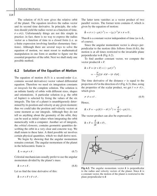
- Page 124 and 125: 116 6. Celestial Mechanics prove (6
- Page 126 and 127: 118 6. Celestial Mechanics in the d
- Page 128 and 129: 120 6. Celestial Mechanics But cons
- Page 130 and 131: 122 6. Celestial Mechanics by the e
- Page 132 and 133: 124 6. Celestial Mechanics Substitu
- Page 134 and 135: 126 6. Celestial Mechanics a cloud
- Page 136 and 137: 128 6. Celestial Mechanics Since th
- Page 138 and 139: 130 6. Celestial Mechanics Exercise
- Page 140 and 141: 132 7. The Solar System Fig. 7.1. (
- Page 142 and 143: 134 7. The Solar System for each ob
- Page 144 and 145: 136 7. The Solar System Fig. 7.5. L
- Page 146 and 147: 138 7. The Solar System Inserting t
- Page 148 and 149: 140 7. The Solar System Therefore o
- Page 150 and 151: 142 7. The Solar System Fig. 7.10.
- Page 152 and 153: 144 7. The Solar System behaves mor
- Page 154 and 155: 146 7. The Solar System Table 7.1.
- Page 156 and 157: 148 7. The Solar System Table 7.2.
- Page 158 and 159: 150 7. The Solar System of the plan
- Page 160 and 161: 152 7. The Solar System If we denot
- Page 162 and 163: 154 7. The Solar System where F⊥
- Page 164 and 165: 156 7. The Solar System Table 7.3.
- Page 166 and 167: 158 7. The Solar System larized fea
- Page 168 and 169: 160 7. The Solar System Fig. 7.26.
- Page 170 and 171: 162 7. The Solar System The outer c
- Page 172 and 173:
164 7. The Solar System Fig. 7.29.
- Page 174 and 175:
166 7. The Solar System Fig. 7.31.
- Page 176 and 177:
168 7. The Solar System weak and co
- Page 178 and 179:
170 7. The Solar System amount of w
- Page 180 and 181:
172 7. The Solar System Fig. 7.37.
- Page 182 and 183:
174 7. The Solar System Fig. 7.39.
- Page 184 and 185:
176 7. The Solar System ter the rin
- Page 186 and 187:
178 7. The Solar System face, most
- Page 188 and 189:
180 7. The Solar System The F ring,
- Page 190 and 191:
182 7. The Solar System Herschel hi
- Page 192 and 193:
184 7. The Solar System Fig. 7.49.
- Page 194 and 195:
186 7. The Solar System Fig. 7.52.
- Page 196 and 197:
188 7. The Solar System liding, sin
- Page 198 and 199:
190 7. The Solar System Fig. 7.56.
- Page 200 and 201:
192 7. The Solar System Fig. 7.59.
- Page 202 and 203:
194 7. The Solar System Fig. 7.62.
- Page 204 and 205:
196 7. The Solar System of this mat
- Page 206 and 207:
198 7. The Solar System Fig. 7.65.
- Page 208 and 209:
200 7. The Solar System Fig. 7.67.
- Page 210 and 211:
202 7. The Solar System Near the po
- Page 212 and 213:
204 7. The Solar System be solved f
- Page 214 and 215:
8. Stellar Spectra All our informat
- Page 216 and 217:
which appears as irregular fluctuat
- Page 218 and 219:
8.2 The Harvard Spectral Classifica
- Page 220 and 221:
ate of ionization is essentially de
- Page 222 and 223:
lines of titanium, scandium and van
- Page 224 and 225:
efore τ = 1, i. e. the radiation i
- Page 226 and 227:
yielding Iν(0,θ)= Sν(τ ∗ ) +
- Page 228 and 229:
222 9. Binary Stars and Stellar Mas
- Page 230 and 231:
224 9. Binary Stars and Stellar Mas
- Page 232 and 233:
226 9. Binary Stars and Stellar Mas
- Page 234 and 235:
10. Stellar Structure The stars are
- Page 236 and 237:
where a = 4σ/c = 7.564 × 10⁻¹⁶
- Page 238 and 239:
where me is the electron mass and N
- Page 240 and 241:
is produced by the proton-proton (p
- Page 242 and 243:
oxygen, which in turn reacts to for
- Page 244 and 245:
According to (4.7), (4.4) and (5.16
- Page 246 and 247:
Example 10.6 The Radiation Pressure
- Page 248 and 249:
11. Stellar Evolution In the preced
- Page 250 and 251:
increases. The stellar surface temp
- Page 252 and 253:
Since stars are most likely to be f
- Page 254 and 255:
Fig. 11.4a-c. Energy transport in t
- Page 256 and 257:
Fig. 11.5. The structure of a massi
- Page 258 and 259:
tract to planetlike brown dwarfs. S
- Page 260 and 261:
Fig. 11.10a-f. Evolution of a low-m
- Page 262 and 263:
Fig. 11.12. The Wolf-Rayet star WR
- Page 264 and 265:
In a neutron capture, a nucleus wit
- Page 266 and 267:
This is several orders of magnitude
- Page 268 and 269:
264 12.TheSun Fig. 12.2. (a) The ro
- Page 270 and 271:
266 12.TheSun according to the heli
- Page 272 and 273:
268 12.TheSun shines into view for
- Page 274 and 275:
270 12.TheSun was established that
- Page 276 and 277:
272 12.TheSun Fig. 12.11. In pairs
- Page 278 and 279:
274 12.TheSun Fig. 12.15. (a) Quies
- Page 280 and 281:
276 12.TheSun Fig. 12.17. An X-ray
- Page 282 and 283:
13. Variable Stars Stars with chang
- Page 284 and 285:
Fig. 13.3. The variation of brightn
- Page 286 and 287:
Fig. 13.5. The lightcurve of a long
- Page 288 and 289:
duced when the carbon condenses int
- Page 290 and 291:
13.3 Eruptive Variables Fig. 13.12.
- Page 292 and 293:
Fig. 13.15. Supernova 1987A in the
- Page 294 and 295:
14. Compact Stars In astrophysics t
- Page 296 and 297:
about 1.4 M⊙, which is thus the u
- Page 298 and 299:
1968. In the following year it was
- Page 300 and 301:
ditions required for hypernova expl
- Page 302 and 303:
This is greater than the speed of l
- Page 304 and 305:
Fig. 14.12. Scale drawings of 16 bl
- Page 306 and 307:
are (or, in the radio case, have on
- Page 308 and 309:
14.6 Exercises Exercise 14.1 The ma
- Page 310 and 311:
308 15. The Interstellar Medium Fig
- Page 312 and 313:
310 15. The Interstellar Medium R d
- Page 314 and 315:
312 15. The Interstellar Medium pol
- Page 316 and 317:
314 15. The Interstellar Medium Fig
- Page 318 and 319:
316 15. The Interstellar Medium Fig
- Page 320 and 321:
318 15. The Interstellar Medium Tab
- Page 322 and 323:
320 15. The Interstellar Medium Tab
- Page 324 and 325:
322 15. The Interstellar Medium met
- Page 326 and 327:
324 15. The Interstellar Medium
- Page 328 and 329:
326 15. The Interstellar Medium He
- Page 330 and 331:
328 15. The Interstellar Medium Tab
- Page 332 and 333:
330 15. The Interstellar Medium up
- Page 334 and 335:
332 15. The Interstellar Medium hav
- Page 336 and 337:
334 15. The Interstellar Medium len
- Page 338 and 339:
336 15. The Interstellar Medium dro
- Page 340 and 341:
338 15. The Interstellar Medium the
- Page 342 and 343:
340 16. Star Clusters and Associati
- Page 344 and 345:
342 16. Star Clusters and Associati
- Page 346 and 347:
344 16. Star Clusters and Associati
- Page 348 and 349:
17. The Milky Way On clear, moonles
- Page 350 and 351:
Fig. 17.3. The directions to the ga
- Page 352 and 353:
classes of stars are main sequence
- Page 354 and 355:
Fig. 17.9. The size of the volume e
- Page 356 and 357:
lar material similarly moves in the
- Page 358 and 359:
Fig. 17.14. In order to derive Oort
- Page 360 and 361:
Fig. 17.17. The radial velocity as
- Page 362 and 363:
a suitable mass distribution, such
- Page 364 and 365:
esting because it may be a small-sc
- Page 366 and 367:
material constituting the galaxy. I
- Page 368 and 369:
18. Galaxies The galaxies are the f
- Page 370 and 371:
Fig. 18.3. The classification of no
- Page 372 and 373:
18.1 The Classification of Galaxies
- Page 374 and 375:
Fig. 18.7. Compound luminosity func
- Page 376 and 377:
In order to measure the mass at eve
- Page 378 and 379:
length r0 = 1-5 kpc. In Sc galaxies
- Page 380 and 381:
18.4 Dynamics of Galaxies We have s
- Page 382 and 383:
gas. Some normal spirals may have b
- Page 384 and 385:
the Large and Small Magellanic Clou
- Page 386 and 387:
stars are forming and evolving into
- Page 388 and 389:
panion galaxy. The tail is interpre
- Page 390 and 391:
een made at these wavelengths with
- Page 392 and 393:
galaxies in our present neighbourho
- Page 394 and 395:
394 19. Cosmology tographs form an
- Page 396 and 397:
396 19. Cosmology Fig. 19.3. Hubble
- Page 398 and 399:
398 19. Cosmology element after hyd
- Page 400 and 401:
400 19. Cosmology 19.3 Homogeneous
- Page 402 and 403:
402 19. Cosmology The potential ene
- Page 404 and 405:
404 19. Cosmology In an expanding c
- Page 406 and 407:
406 19. Cosmology about 40,000 degr
- Page 408 and 409:
408 19. Cosmology rather slowly. In
- Page 410 and 411:
410 19. Cosmology Fig. 19.15. Corre
- Page 412 and 413:
412 19. Cosmology where Ω0 = ρ0/
- Page 414 and 415:
414 19. Cosmology Example 19.2 Find
- Page 416 and 417:
416 20. Astrobiology According to t
- Page 418 and 419:
418 20. Astrobiology of spiral gala
- Page 420 and 421:
420 20. Astrobiology Fig. 20.2. Bla
- Page 422 and 423:
422 20. Astrobiology reached 10% of
- Page 424 and 425:
424 20. Astrobiology Now panspermia
- Page 426 and 427:
426 20. Astrobiology 20.9 Detecting
- Page 428 and 429:
428 20. Astrobiology cles that we s
- Page 430 and 431:
Appendices 431
- Page 432 and 433:
Ellipse. Equation in rectangular co
- Page 434 and 435:
A and B can be determined graphical
- Page 436 and 437:
When using matrix formalism it is c
- Page 438 and 439:
Similarly, a volume integral I = f
- Page 440 and 441:
B. Theory of Relativity Albert Eins
- Page 442 and 443:
time interval between the events is
- Page 444 and 445:
C. Tables Table C.1. SI basic units
- Page 446 and 447:
Table C.6. The Sun Property Symbol
- Page 448 and 449:
Table C.11. Osculating elements of
- Page 450 and 451:
Discoverer Year of a Psid e i r M
- Page 452 and 453:
Table C.16. Periodic comets with se
- Page 454 and 455:
Table C.17 (continued) C. Tables Na
- Page 456 and 457:
C. Tables Table C.19. Some double s
- Page 458 and 459:
Table C.22. Optically brightest gal
- Page 460 and 461:
Table C.23 (continued) Abbreviation
- Page 462 and 463:
C. Tables Table C.26. Millimetre an
- Page 464 and 465:
Table C.27 (continued) Satellite La
- Page 466 and 467:
468 Answers to Exercises 6.2 a = 1.
- Page 468 and 469:
470 Answers to Exercises Chapter 17
- Page 470 and 471:
472 Further Reading Morrison (ed.):
- Page 472 and 473:
474 Further Reading Maps and Catalo
- Page 474 and 475:
Name and Subject Index A aberration
- Page 476 and 477:
coherent radiation 95 Cold Dark Mat
- Page 478 and 479:
forbidden transition 101, 332 four-
- Page 480 and 481:
Kellman, Edith 212 Kepler’s equat
- Page 482 and 483:
nautical mile 15 nautical triangle
- Page 484 and 485:
Reber, Grote 69 recombination 95, 9
- Page 486 and 487:
synchronous rotation 135 synchrotro
- Page 488 and 489:
Colour Supplement 491
- Page 490 and 491:
Plate 14. The first view from the s
- Page 492 and 493:
Plate 1 Plate 2 Colour Supplement 4
- Page 494 and 495:
Plate 6 Plate 5 Colour Supplement 4
- Page 496 and 497:
Plate 9 Colour Supplement Plate 10
- Page 498 and 499:
Plate 14 Colour Supplement Plate 13
- Page 500 and 501:
Plate 17 Colour Supplement Plate 18
- Page 502 and 503:
Plate 23 Plate 24 Colour Supplement
- Page 504 and 505:
Colour Supplement Plate 29 507
- Page 506 and 507:
Plate 31 Colour Supplement Plate 32