Regularization of the AVO inverse problem by means of a ...

CHAPTER 2. AVO MODELING 11
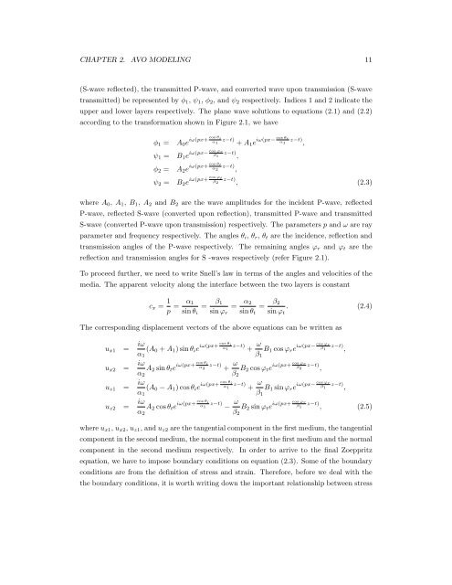
(S-wave reflected), the transmitted P-wave, and converted wave upon transmission (S-wave
transmitted) be represented by φ1, ψ1, φ2, and ψ2 respectively. Indices 1 and 2 indicate the
upper and lower layers respectively. The plane wave solutions to equations (2.1) and (2.2)
according to the transformation shown in Figure 2.1, we have
φ1 = A0e iω(px+ cos θi cos θr
α z−t) iω(px−
1 α z−t)
+ A1e 1 ,
cos ϕr
iω(px− β z−t)
ψ1 = B1e 1 ,
φ2 = A2e iω(px+ cos θ t
α 2 z−t) ,
ψ2 = B2e iω(px+ cos ϕ t
β 2 z−t) , (2.3)
where A0, A1, B1, A2 and B2 are the wave amplitudes for the incident P-wave, reflected
P-wave, reflected S-wave (converted upon reflection), transmitted P-wave and transmitted
S-wave (converted P-wave upon transmission) respectively. The parameters p and ω are ray
parameter and frequency respectively. The angles θi, θr, θt are the incidence, reflection and
transmission angles of the P-wave respectively. The remaining angles ϕr and ϕt are the
reflection and transmission angles for S -waves respectively (refer Figure 2.1).
To proceed further, we need to write Snell’s law in terms of the angles and velocities of the
media. The apparent velocity along the interface between the two layers is constant
cx = 1 α1
= =
p sin θi
β1
sin ϕr
= α2
=
sin θt
β2
. (2.4)
sin ϕt
The corresponding displacement vectors of the above equations can be written as
ux1 = iω
ux2 = iω
uz1 = iω
uz2 = iω
(A0 + A1) sin θie iω(px+ cos θ i
α 1 z−t) + ω
cos ϕr
iω(px− β z−t)
B1 cos ϕre 1 ,
α1
β1
A2 sin θte
α2
iω(px+ cos θi α z−t) ω
cos ϕr
iω(px+
2 β z−t)
+ B2 cos ϕte 2 ,
β2
(A0 − A1) cos θie
α1
iω(px+ cos θi α z−t) ω
cos ϕr
iω(px−
1 β z−t)
+ B1 sin ϕre 1 ,
β1
A2 cos θte
α2
iω(px+ cos θi α z−t) ω
cos ϕr
iω(px+
1 β z−t)
− B2 sin ϕte 1 , (2.5)
β2
where ux1, ux2, uz1, and uz2 are the tangential component in the first medium, the tangential
component in the second medium, the normal component in the first medium and the normal
component in the second medium respectively. In order to arrive to the final Zoeppritz
equation, we have to impose boundary conditions on equation (2.3). Some of the boundary
conditions are from the definition of stress and strain. Therefore, before we deal with the
the boundary conditions, it is worth writing down the important relationship between stress