Regularization of the AVO inverse problem by means of a ...

CHAPTER 3. BAYESIAN INVERSION APPROACH AND ALGORITHMS 28
where Σ is a parameter covariance matrix. The univariate version of equation (3.3) has the
form
P (x|σ) = 1
(x − µ)2
√ exp −
2πσ 2σ2
, (3.4)
where σ is the standard deviation of the model parameter, x.
Multivariate t distribution
The Multivariate t distribution is generalization of classical univariate Student t distribution
which is another type of distribution useful for multivariate analysis (Chauanhai, 1994). It is
known by a typical nature having heavy tails as compared to exponential distributions and
they are more realistic in real world (Nadarajah and Korz, 2008). The general Multivariate
t distribution is given by,
P (x i |µ, Ψ, ν) =
Γ( ν+p
2 )|Ψ|−1/2
(πν) p/2Γ( ν 1
2 )[1 + ν (xi − µ) T Ψ−1 (xi − µ)] (ν+p)
2
. (3.5)
The model x i is a p dimensional vector whose elements are in the range −∞ < xj < ∞ for
j = 1, 2, 3 , ..., p and having a p dimensional vector center, µ. The degree of correlation is
represented by a p×p dimensional scale matrix, Ψ. The parameter ν is the degree of freedom
or the shaping parameter which controls the shape of the distribution. Before discussing
the multivariate case, it is easier to see the Univariate t distribution in comparison with the
Univariate Gaussian distribution. For p = 1, the Univariate form of equation (3.6) has the
form .
P (x|µ, σ, ν) =
Γ( ν+1
2 )
σ √ πνΓ( ν 1
2 )[1 + νσ2 (x − µ) 2 ] (ν+1)
2
, (3.6)
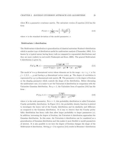
where σ is the scale parameter. For ν = 1, this probability distribution is called Univariate
Cauchy probability distribution. In Figure (3.1), the probability density function is plotted
to investigate the heavy tail of the Cauchy distribution and its similarity and difference
as compared to the Gaussian distribution. It is easy to observe that the Cauchy proba-
bility distribution has heavy tails that allow larger probability to larger parameters (x).
In addition, increasing the degree of freedom, the Univariate t distribution approaches the
Gaussian distribution. In this sense, the Univariate t distribution can be considered as a
generalization of Gaussian distribution and this makes it more flexible to model parameters
of interest. It is also possible to see how the degree of freedom changes the shape of the
Multivariate t distribution. Setting p = 2 in equation (3.6) results in Bivariate t distribution