Regularization of the AVO inverse problem by means of a ...
Regularization of the AVO inverse problem by means of a ...
Regularization of the AVO inverse problem by means of a ...

You also want an ePaper? Increase the reach of your titles
YUMPU automatically turns print PDFs into web optimized ePapers that Google loves.
CHAPTER 3. BAYESIAN INVERSION APPROACH AND ALGORITHMS 36<br />
solution is given <strong>by</strong><br />
m = (L T C −1<br />
d L + µQ(m))−1L T C −1<br />
d<br />
d. (3.19)<br />
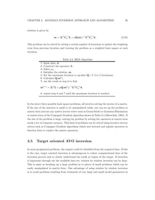
This <strong>problem</strong> can be solved <strong>by</strong> setting a certain number <strong>of</strong> iterations to update <strong>the</strong> weighting<br />
term from previous iteration and treating <strong>the</strong> <strong>problem</strong> as a weighted least square at each<br />
iteration.<br />
Table 3.3: IRLS Algorithm<br />
1: Input data, d.<br />
2: Construct <strong>the</strong> operator, L.<br />
3: Select µh.<br />
4: Initialize <strong>the</strong> solution, m.<br />
5: Set <strong>the</strong> maximum iteration to up-date Q ( ∼ = 3 to 5 iterations).<br />
6: Calculate Q(mk ),<br />
7: use <strong>the</strong> result in step 6 to find,<br />
m k+1 = (L T L + µQ(m k )) −1 L T C −1<br />
d d,<br />
8: repeat step 6 and 7 until <strong>the</strong> maximum iteration is reached.<br />
In <strong>the</strong> above three possible least square <strong>problem</strong>s, all involves solving <strong>the</strong> <strong>inverse</strong> <strong>of</strong> a matrix.<br />
If <strong>the</strong> size <strong>of</strong> <strong>the</strong> matrices is small to be manipulated easily, one can set up <strong>the</strong> <strong>problem</strong> in<br />
matrix form and use any matrix <strong>inverse</strong> solver such as Gauss-Seidel or Gaussian-Elimination<br />
or matrix form <strong>of</strong> <strong>the</strong> Conjugate Gradient algorithm shown in Table 3.4 (Shewchuk, 1994). If<br />
<strong>the</strong> size <strong>of</strong> <strong>the</strong> <strong>problem</strong> is large, solving <strong>the</strong> <strong>problem</strong> <strong>by</strong> setting <strong>the</strong> operators in matrix form<br />
needs a lot <strong>of</strong> computer memory. This kind <strong>of</strong> <strong>problem</strong>s can be solved using iterative <strong>inverse</strong><br />
solvers such as Conjugate Gradient algorithms which uses forward and adjoint operators in<br />
function form to replace <strong>the</strong> matrix operators.<br />
3.5 Target oriented <strong>AVO</strong> inversion<br />
In most geophysical <strong>problem</strong>s, <strong>the</strong> targets could be identified from <strong>the</strong> acquired data. If this<br />
is <strong>the</strong> case, target oriented inversion is advantageous to reduce computational time <strong>of</strong> <strong>the</strong><br />
inversion process and to clearly understand <strong>the</strong> result at region <strong>of</strong> <strong>the</strong> target. If inversion<br />
is important through out <strong>the</strong> available data set, window <strong>by</strong> window inversion can be done.<br />
This is same as breaking up a large <strong>problem</strong> in to pieces <strong>of</strong> small <strong>problem</strong>s which can be<br />
easily manipulated in matrix form. One advantage <strong>of</strong> using window <strong>by</strong> window inversion<br />
is to avoid <strong>problem</strong>s resulting from treatment <strong>of</strong> very large and small model parameters in