Regularization of the AVO inverse problem by means of a ...

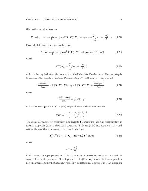
CHAPTER 4. TWO-TERM AVO INVERSION 44
this particular prior becomes
P (mf |d) ∝ exp{− 1
2 (d − Lf mf ) T Υ T C −1
d Υ(d − Lf
2N
mf ) − ln(1 + (
i=1
mi f
σ )2 }. (4.20)
From which follows, the objective function
where
J uc (mf ) = 1
2 (d − Lf mf ) T Υ T C −1
d Υ(d − Lf mf ) + R uc (mf )} (4.21)
R uc (mf ) =
2N
i=1
ln(1 + ( mi f
σ )2 ) (4.22)
which is the regularization that comes from the Univariate Cauchy prior. The next step is
to minimize the objective function. Differentiating J uc with respect to mf , we get
where
∂J uc (mf )
∂mf
= L T f Υ T C −1
d ΥLf mf − L T f Υ T C −1
d Υd + ∂Ruc (mf )
∂R uc (mf )
∂mf
= 2
Quc
σ2 f mf
∂mf
and the matrix Q uc
f is a (2N) × (2N) diagonal matrix whose elements are
[(Q uc
f )kk] = 1 +
, (4.23)
(4.24)
k
m 2−1 f
. (4.25)
σ
The detail derivation for generalized Multivariate t distribution and the regularization is
given in Appendix (A.2). Substituting equations (4.16) and (4.24) into equation (4.23), and
setting the resulting expression to zero, we finally have
where
(L T f Υ T ΥLf + µ uc Q uc
f )mf = L T f Υ T ΥLf d, (4.26)
µ uc ∼ 2σ2 d
σ 2
which means the hyper-parameter µ uc is in the order of ratio of the noise variance and the
square of the scale parameter. The dependence of Q uc
f on mf makes the inverse problem
non-linear unlike using the Gaussian probability distribution as a prior. The IRLS algorithm