Regularization of the AVO inverse problem by means of a ...

CHAPTER 3. BAYESIAN INVERSION APPROACH AND ALGORITHMS 32
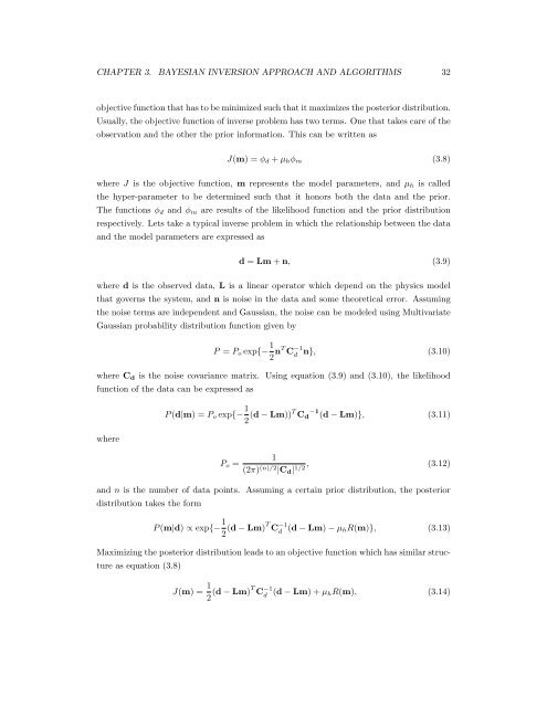
objective function that has to be minimized such that it maximizes the posterior distribution.
Usually, the objective function of inverse problem has two terms. One that takes care of the
observation and the other the prior information. This can be written as
J(m) = φd + µhφm
(3.8)
where J is the objective function, m represents the model parameters, and µh is called
the hyper-parameter to be determined such that it honors both the data and the prior.
The functions φd and φm are results of the likelihood function and the prior distribution
respectively. Lets take a typical inverse problem in which the relationship between the data
and the model parameters are expressed as
d = Lm + n, (3.9)
where d is the observed data, L is a linear operator which depend on the physics model
that governs the system, and n is noise in the data and some theoretical error. Assuming
the noise terms are independent and Gaussian, the noise can be modeled using Multivariate
Gaussian probability distribution function given by
P = Po exp{− 1
2 nT C −1
d n}, (3.10)
where Cd is the noise covariance matrix. Using equation (3.9) and (3.10), the likelihood
function of the data can be expressed as
where
P (d|m) = Po exp{− 1
2 (d − Lm))T Cd −1 (d − Lm)}, (3.11)
Po =
1
(2π) (n)/2 , (3.12)
|Cd| 1/2
and n is the number of data points. Assuming a certain prior distribution, the posterior
distribution takes the form
P (m|d) ∝ exp{− 1
2 (d − Lm)T C −1
d (d − Lm) − µhR(m)}, (3.13)
Maximizing the posterior distribution leads to an objective function which has similar struc-
ture as equation (3.8)
J(m) = 1
2 (d − Lm)T C −1
d (d − Lm) + µhR(m), (3.14)