Regularization of the AVO inverse problem by means of a ...

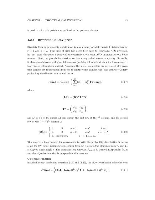
CHAPTER 4. TWO-TERM AVO INVERSION 45
is used to solve this problem as outlined in the previous chapter.
4.2.4 Bivariate Cauchy prior
Bivariate Cauchy probability distribution is also a family of Multivariate t distribution for
ν = 1 and p = 2. This kind of prior has never been used to constraint AVO inversion.
In this thesis, this prior is proposed to constraint a two term AVO inversion for two basic
reasons. First, the probability distribution has a long tailed nature to sparsity. Secondly,
it allows to add some geological information (well-log information) via a 2 × 2 scale matrix
(correlation information matrix). Assuming the model parameters are correlated at a given
time sample but independent from one to another time sample, the joint Bivariate Cauchy
probability distribution can be written as
where
P (mf ) = Pm0 exp[− 3
2
N
i=1
ln(1 + m T f (Φ bc
f ) i mf )], (4.27)
(Φ bc
f ) i = (D i ) T Ψ bc D i , (4.28)
Ψ bc =
ψ11 ψ12
ψ21 ψ22
, (4.29)
and D i is a 3 × 3N matrix all zero except the first row at the i th column, and the second
row at the (i + N) th column i.e
[D i nl] =
⎧
⎪⎨
⎪⎩
1, if n = 1 and l = i
1, if n = 2 and l = i + N,
0, otherwise, i = 1, 2, 3, .., N.
(4.30)
This matrix is incorporated for convenience to write the probability distribution in terms
of all the 2N model parameters in column form i.e it selects two elements from rα and rβ
at a given time sample i. The normalization constant, Pm0, is as defined in Appendix (A.2)
and the objective function is independent this constant.
Objective function
In a similar way, combining equations (4.9) and (4.27), the objective function takes the form
J bc (mf ) = 1
2 (Υ(d − Lf mf )) T C −1
d Υ(d − Lf mf )) + R bc (mf ), (4.31)