Regularization of the AVO inverse problem by means of a ...

More documents

Recommendations

Info

CHAPTER 2. AVO MODELING 18 2.3.5 Smith and Gidlow’s approximation Smith and Gidlow (2003) rearranged the Aki and Richards’s approximation as Rpp(θi) = 1 2 (∆α ∆ρ + α ρ ) − 2γ2 sin 2 θ(2 ∆β β ∆ρ 1 + ) + ρ 2 tan2 θ ∆α . (2.31) α Further, under the assumption that density follows Gardner’s relationship, equation (1.1), they put Rpp as only two terms where the model parameters are the P-wave reflectivity and S-wave reflectivity. This equation is given by Rpp(θi) = 1 2 (1 + a + tan2 θ − 4aγ 2 sin 2 θ) ∆α α − 4γ2 sin 2 θ ∆β β (2.32) where a = 0.25 is constant in Gardner’s equation, equation (1.1). In addition to the above given approximation, they also define what is called fluid factor making use of Castagna’s equation, equation (1.3). The fluid factor is defied as ∆F = ∆α α − cγ ∆β β (2.33) where c = 1.16 is gradient of the Castagna’s equation. The equality in this equation don’t hold for hydrocarbon reservoirs and it is useful indicator for hydrocarbon indicator by analyzing the deviation from this relationship (Castagna et al., 1998). 2.3.6 Fatti’s approximation This approximation was proposed by Fatti et al. (1994) by rearranging the Aki and Richards’s approximation and expressing it in terms of P-wave impedance, S-wave impedance, and density reflectivity. The resulting equation has the form where Rpp(θi) = 1 2 (1 + tan2 θ) ∆Ip − 4γ Ip 2 sin 2 θ ∆Is − Is 1 2 (tan2 θ − 4γ 2 sin 2 θ) ∆ρ , (2.34) ρ ∆Ip Ip ∆Is Is = α2ρ2 − α1ρ1 , α2ρ2 + α1ρ1 = β2ρ2 − β1ρ1 . (2.35) β2ρ2 + β1ρ1
CHAPTER 2. AVO MODELING 19 Assuming very small change in density, the last term in equation (2.34) cab be ignored and results in the following expression Rpp(θi) = 1 2 (1 + tan2 θ) ∆Ip Ip − 4γ 2 sin 2 θ ∆Is . (2.36) The model parameters in this equation are the P-wave and S-wave impedance. This approximation is used in Chapter 4 for the two-term AVO inversion problem. 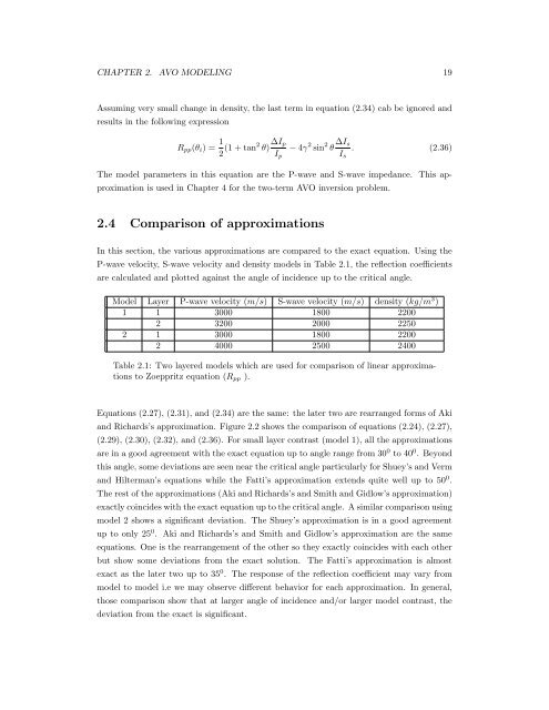2.4 Comparison of approximations In this section, the various approximations are compared to the exact equation. Using the P-wave velocity, S-wave velocity and density models in Table 2.1, the reflection coefficients are calculated and plotted against the angle of incidence up to the critical angle. Model Layer P-wave velocity (m/s) S-wave velocity (m/s) density (kg/m 3 ) 1 1 3000 1800 2200 2 3200 2000 2250 2 1 3000 1800 2200 2 4000 2500 2400 Table 2.1: Two layered models which are used for comparison of linear approximations to Zoeppritz equation (Rpp ). Equations (2.27), (2.31), and (2.34) are the same: the later two are rearranged forms of Aki and Richards’s approximation. Figure 2.2 shows the comparison of equations (2.24), (2.27), (2.29), (2.30), (2.32), and (2.36). For small layer contrast (model 1), all the approximations are in a good agreement with the exact equation up to angle range from 30 0 to 40 0 . Beyond this angle, some deviations are seen near the critical angle particularly for Shuey’s and Verm and Hilterman’s equations while the Fatti’s approximation extends quite well up to 50 0 . The rest of the approximations (Aki and Richards’s and Smith and Gidlow’s approximation) exactly coincides with the exact equation up to the critical angle. A similar comparison using model 2 shows a significant deviation. The Shuey’s approximation is in a good agreement up to only 25 0 . Aki and Richards’s and Smith and Gidlow’s approximation are the same equations. One is the rearrangement of the other so they exactly coincides with each other but show some deviations from the exact solution. The Fatti’s approximation is almost exact as the later two up to 35 0 . The response of the reflection coefficient may vary from model to model i.e we may observe different behavior for each approximation. In general, those comparison show that at larger angle of incidence and/or larger model contrast, the deviation from the exact is significant. Is
Page 1 and 2: University of Alberta Regularizatio
Page 3 and 4: Abstract Amplitude Variation with O
Page 5 and 6: Contents 1 Introduction 1 1.1 Forwa
Page 7 and 8: 5 Three-term AVO Inversion 55 5.1 I
Page 9 and 10: List of Figures 1.1 A simple diagra
Page 11 and 12: 5.3 (a) P-wave reflectivity (RMSEA
Page 13 and 14: CHAPTER 1 Introduction The reflecti
Page 15 and 16: CHAPTER 1. INTRODUCTION 3 ! !!!!!!!
Page 17 and 18: CHAPTER 1. INTRODUCTION 5 1.4.1 Rel
Page 19 and 20: CHAPTER 1. INTRODUCTION 7 three-ter
Page 21 and 22: 2.1 Introduction CHAPTER 2 AVO Mode
Page 23 and 24: CHAPTER 2. AVO MODELING 11 (S-wave
Page 25 and 26: CHAPTER 2. AVO MODELING 13 At this
Page 27 and 28: CHAPTER 2. AVO MODELING 15 The resu
Page 29: CHAPTER 2. AVO MODELING 17 2.3.3 Sh
Page 33 and 34: CHAPTER 2. AVO MODELING 21 Reflecti
Page 35 and 36: CHAPTER 2. AVO MODELING 23 ! !"# %$
Page 37 and 38: CHAPTER 2. AVO MODELING 25 can be r
Page 39 and 40: CHAPTER 3. BAYESIAN INVERSION APPRO
Page 51 and 52: 4.1 Introduction CHAPTER 4 Two-term
Page 53 and 54: CHAPTER 4. TWO-TERM AVO INVERSION 4
Page 67 and 68: 5.1 Introduction CHAPTER 5 Three-te
Page 69 and 70: CHAPTER 5. THREE-TERM AVO INVERSION
Page 81 and 82:
CHAPTER 5. THREE-TERM AVO INVERSION
Page 83 and 84:
Page 85 and 86:
Page 87 and 88:
Page 89 and 90:
CHAPTER 6. CONCLUSIONS 77 two terms
Page 91 and 92:
Bibliography Aki, K. and P. G. Rich
Page 93 and 94:
BIBLIOGRAPHY 81 Sacchi, M.D. and T.
Page 95 and 96:
APPENDIX A Multivariate t distribut
Page 97 and 98:
APPENDIX A. MULTIVARIATE T DISTRIBU
Page 99 and 100:
APPENDIX B EM Algorithm B.1 EM-Algo
Page 101:
APPENDIX C Calculation of root mean
show all

Regularization of the AVO inverse problem by means of a ...

Create successful ePaper yourself

Delete template?

Save as template?